Error Rates
Last updated on 2025-09-23 | Edit this page
Overview
Questions
- Why are type I and II error rates a problem in inferential statistics?
- What is Family Wise Error Rate, and why is it a concern in high throughput data?
Objectives
- Calculate error rates in simulated data.
- Calculate the number of false positives that occur in a given data set.
- Define family wise error rates.
Error Rates
Throughout this section we will be using the type I error and type II error terminology. We will also refer to them as false positives and false negatives respectively. We also use the more general terms specificity, which relates to type I error, and sensitivity, which relates to type II errors.
Types of Error
Whenever we perform a statistical test, we are aware that we may make a mistake. This is why our p-values are not 0. Under the null, there is always a positive, perhaps very small, but still positive chance that we will reject the null when it is true. If the p-value is 0.05, it will happen 1 out of 20 times. This error is called type I error by statisticians.
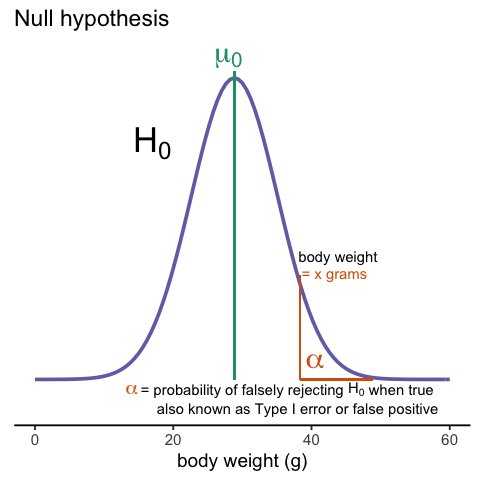
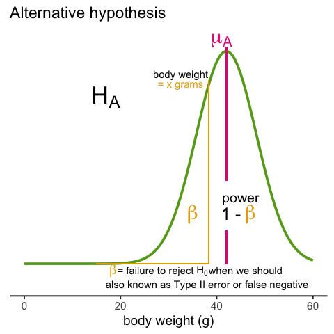
A type I error is defined as rejecting the null when we should not. This is also referred to as a false positive. So why do we then use 0.05? Shouldn’t we use 0.000001 to be really sure? The reason we don’t use infinitesimal cut-offs to avoid type I errors at all cost is that there is another error we can commit: to not reject the null when we should. This is called a type II error or a false negative.
In the context of high-throughput data we can make several type I errors and several type II errors in one experiment, as opposed to one or the other as seen in Chapter 1. In this table, we summarize the possibilities using the notation from the seminal paper by Benjamini-Hochberg:
| Called significant | Not called significant | Total | |
|---|---|---|---|
| Null True | \(V\) | \(m_0-V\) | \(m_0\) |
| Alternative True | \(S\) | \(m_1-S\) | \(m_1\) |
| True | \(R\) | \(m-R\) | \(m\) |
To describe the entries in the table, let’s use as an example a dataset representing measurements from 10,000 genes, which means that the total number of tests that we are conducting is: \(m=10,000\). The number of genes for which the null hypothesis is true, which in most cases represent the “non-interesting” genes, is \(m_0\), while the number of genes for which the null hypothesis is false is \(m_1\). For this we can also say that the alternative hypothesis is true. In general, we are interested in detecting as many as possible of the cases for which the alternative hypothesis is true (true positives), without incorrectly detecting cases for which the null hypothesis is true (false positives). For most high-throughput experiments, we assume that \(m_0\) is much greater than \(m_1\). For example, we test 10,000 expecting 100 genes or less to be interesting. This would imply that \(m_1 \leq 100\) and \(m_0 \geq 19,900\).
Throughout this chapter we refer to features as the units being tested. In genomics, examples of features are genes, transcripts, binding sites, CpG sites, and SNPs. In the table, \(R\) represents the total number of features that we call significant after applying our procedure, while \(m-R\) is the total number of genes we don’t call significant. The rest of the table contains important quantities that are unknown in practice.
- \(V\) represents the number of type I errors or false positives. Specifically, \(V\) is the number of features for which the null hypothesis is true, that we call significant.
- \(S\) represents the number of true positives. Specifically, \(S\) is the number of features for which the alternative is true, that we call significant.
This implies that there are \(m_1-S\) type II errors or false negatives and \(m_0-V\) true negatives. Keep in mind that if we only ran one test, a p-value is simply the probability that \(V=1\) when \(m=m_0=1\). Power is the probability of \(S=1\) when \(m=m_1=1\). In this very simple case, we wouldn’t bother making the table above, but now we show how defining the terms in the table helps for the high-dimensional setting.
Data example
Let’s compute these quantities with a data example. We will use a Monte Carlo simulation using our mice data to imitate a situation in which we perform tests for 10,000 different fad diets, none of them having an effect on weight. This implies that the null hypothesis is true for diets and thus \(m=m_0=10,000\) and \(m_1=0\). Let’s run the tests with a sample size of \(N=12\) and compute \(R\). Our procedure will declare any diet achieving a p-value smaller than \(\alpha=0.05\) as significant.
R
set.seed(1)
population = unlist( read.csv(file = "./data/femaleControlsPopulation.csv") )
alpha <- 0.05
N <- 12
m <- 10000
pvals <- replicate(m,{
  control = sample(population,N)
  treatment = sample(population,N)
  t.test(treatment,control)$p.value
})
Although in practice we do not know the fact that no diet works, in this simulation we do, and therefore we can actually compute \(V\) and \(S\). Because all null hypotheses are true, we know, in this specific simulation, that \(V=R\). Of course, in practice we can compute \(R\) but not \(V\).
R
sum(pvals < 0.05)
OUTPUT
[1] 409These many false positives are not acceptable in most contexts.
Here is more complicated code showing results where 10% of the diets are effective with an average effect size of \(\Delta= 3\) ounces. Studying this code carefully will help us understand the meaning of the table above. First let’s define the truth:
R
alpha <- 0.05
N <- 12
m <- 10000
p0 <- 0.90 ##10% of diets work, 90% don't
m0 <- m * p0
m1 <- m - m0
nullHypothesis <- c( rep(TRUE, m0), rep(FALSE, m1))
delta <- 3
Now we are ready to simulate 10,000 tests, perform a t-test on each, and record if we rejected the null hypothesis or not:
R
set.seed(1)
calls <- sapply(1:m, function(i){
  control <- sample(population, N)
  treatment <- sample(population, N)
  if(!nullHypothesis[i]) treatment <- treatment + delta
  ifelse( t.test(treatment, control)$p.value < alpha,
          "Called Significant",
          "Not Called Significant")
})
Because in this simulation we know the truth (saved in
nullHypothesis), we can compute the entries of the
table:
R
null_hypothesis <- factor(nullHypothesis, levels=c("FALSE", "TRUE"))
table(null_hypothesis, calls)
OUTPUT
               calls
null_hypothesis Called Significant Not Called Significant
          FALSE                553                    447
          TRUE                 361                   8639
The first column of the table above shows us \(V\) and \(S\). Note that \(V\) and \(S\) are random variables. If we run the simulation repeatedly, these values change. Here is a quick example:
R
B <- 10 ##number of simulations
VandS <- replicate(B,{
  calls <- sapply(1:m, function(i){
    control <- sample(population, N)
    treatment <- sample(population, N)
    if(!nullHypothesis[i]) treatment <- treatment + delta
    t.test(treatment, control)$p.val < alpha
  })
  cat("V =",sum(nullHypothesis & calls), "S =",sum(!nullHypothesis & calls),"\n")
  c(sum(nullHypothesis & calls),sum(!nullHypothesis & calls))
  })
OUTPUT
V = 373 S = 540
V = 375 S = 553
V = 386 S = 545
V = 396 S = 565
V = 373 S = 532
V = 355 S = 541
V = 372 S = 501
V = 376 S = 522
V = 355 S = 570
V = 388 S = 506
This motivates the definition of error rates. We can, for example, estimate probability that \(V\) is larger than 0. This is interpreted as the probability of making at least one type I error among the 10,000 tests. In the simulation above, \(V\) was much larger than 1 in every single simulation, so we suspect this probability is very practically 1. When \(m=1\), this probability is equivalent to the p-value. When we have a multiple tests situation, we call it the Family Wise Error Rate (FWER) and it relates to a technique that is widely used: The Bonferroni Correction.
Discussion
Refer to the confusion matrix below showing false positive and false
negative rates, along with specificity and sensitivity. Turn to a
partner and explain the following:
How is specificity related to Type I error and false positive
rates?
How is sensitivity related to Type II error and false negative
rates?
When you are finished discussing, share with the group in the
collaborative document.
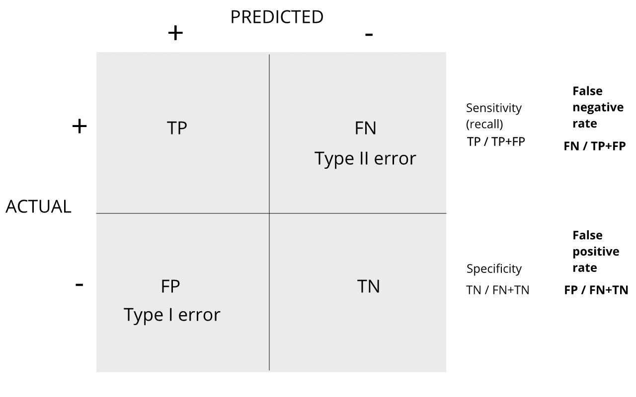
For more on this, see Classification evaluation by J. Lever, M. Krzywinski and N. Altman in Nature Methods 13, 603-604 (2016).
- Type 1 and Type II error are complementary concerns in data analysis. The reason we don’t have extremely strict cutoffs for alpha is because we don’t want to miss finding true positive results.
- It is possible to calculate the probability of finding at least one false positive result when conducting multiple inferential tests. This is the Family Wise Error Rate.