Experimental designs
Overview
Teaching: 0 min
Exercises: 0 minQuestions
What are my experimental units?
How will treatments be assigned?
What are some types of experimental design?
Objectives
Identify different sources of error to increase accuracy and minimize sources of error
Select an appropriate experimental design for a specific study
library(downloader)
Warning: package 'downloader' was built under R version 4.0.2
url <- "https://raw.githubusercontent.com/smcclatchy/dals-inference/gh-pages/data/bodyWeights.csv"
filename <- "bodyWeights.csv"
if(!file.exists(filename)) download(url,destfile=filename)
library(dplyr)

# Read in DO850 body weight data.
dat <- read.csv("bodyWeights.csv")
A designed experiment is a strategic attempt to answer a research question or problem. Experiments give us a way to compare effects of two or more treatments of interest. When well-designed, experiments minimize any bias in this comparison. When we control experiments, that control gives us the ability to make stronger inferences about the differences we see in the experiment. Specifically, experiments allow us to make inferences about causation. Sample research questions that follow from these questions are given below.
- Does
affect condition X in humans? - Does
affect phenotype Y in mice?
The research question suggests how an experiment might be carried out to find an answer. In the questions above, the treatments are either a drug or a diet. The experimental units are those things to which we apply treatments.
Discussion
What are the experimental units in each of the research questions above?
Solution
1). Research question: Does
affect condition X in humans? Experimental unit: Individual person on drug or placebo 2). Research question: Does affect phenotype Y in mice? Experimental unit: Cage of mice on treatment or control diet
Defining the experimental unit is not necessarily straightforward. To define the experimental unit, consider that an experimental unit should be able to receive any treatment. In the second example, all mice in a cage must receive either the treatment or the control diet. In this case the cage is the experimental unit. Each individual mouse is a measurement unit since we would measure the response of each individual mouse to the diet. We don’t measure how the entire cage of mice responds to the diet as a whole, though. Individual mice are the measurement units, while the cage is an experimental unit since all mice in the cage receive the same treatment.
Well-designed experiments are characterized by three features: randomization, replication, and control. These features help to minimize the impact of experimental error and factors not under study.
Randomization
In a randomized experiment, the investigators randomly assign subjects to treatment and control groups in order to minimize bias and moderate experimental error. A random number table or generator can be used to assign random numbers to experimental units (the unit or subject tested upon) so that any experimental unit has equal chances of being assigned to treatment or control. The random number then determines to which group an experimental unit belongs. For example, odd-numbered experimental units could go in the treatment group, and even-numbered experimental units in the control group.
Here is an example of randomization using a random number generator. If the random number is even, the sample is assigned to the control group. If odd, the sample is assigned to the treatment group.
sample_id <- LETTERS
random_number <- sample(x = 100, size = 26)

# %% is the modulo operator, which returns the remainder from division
group <- ifelse(random_number %% 2 == 0, "control", "treatment")
df1 <- data.frame(sample_id, random_number, group)
df1
   sample_id random_number     group
1          A            61 treatment
2          B             9 treatment
3          C            89 treatment
4          D            88   control
5          E            40   control
6          F             8   control
7          G            44   control
8          H            75 treatment
9          I            77 treatment
10         J            52   control
11         K            80   control
12         L            84   control
13         M            64   control
14         N            17 treatment
15         O            23 treatment
16         P            27 treatment
17         Q            85 treatment
18         R            63 treatment
19         S             6   control
20         T            86   control
21         U            20   control
22         V            50   control
23         W            51 treatment
24         X            94   control
25         Y            58   control
26         Z            57 treatment
This might produce unequal numbers between treatment and control groups. It isn’t necessary to have equal numbers, however, sensitivity (the true positive rate, or ability to detect an effect when it truly exists) is maximized when sample numbers are equal.
table(df1$group)
  control treatment
       14        12
To randomly assign samples to groups with equal numbers, you can do the following.
# place IDs and random numbers in data frame
df1_equal <- data.frame(sample_id, random_number)

# sort by random numbers (not by sample IDs)
df1_equal <- df1_equal[order(random_number),]

# now assign to treatment or control groups
treatment <- sort(rep(x = c("control", "treatment"), times = 13))
df1_equal <- cbind(df1_equal, treatment)
row.names(df1_equal) <- 1:26
df1_equal
   sample_id random_number treatment
1          S             6   control
2          F             8   control
3          B             9   control
4          N            17   control
5          U            20   control
6          O            23   control
7          P            27   control
8          E            40   control
9          G            44   control
10         V            50   control
11         W            51   control
12         J            52   control
13         Z            57   control
14         Y            58 treatment
15         A            61 treatment
16         R            63 treatment
17         M            64 treatment
18         H            75 treatment
19         I            77 treatment
20         K            80 treatment
21         L            84 treatment
22         Q            85 treatment
23         T            86 treatment
24         D            88 treatment
25         C            89 treatment
26         X            94 treatment
Discussion
Why not assign treatment and control groups to samples in alphabetical order?
Did we really need a random number generator to obtain randomized equal groups?Solution
1). Scenario: One technician processed samples A through M, and a different technician processed samples N through Z.
2). Another scenario: Samples A through M were processed on a Monday, and samples N through Z on a Tuesday.
3). Yet another scenario: Samples A through M were from one strain, and samples N through Z from a different strain.
4). Yet another scenario: Samples with consecutive ids were all sibling groups. For example, samples A, B and C were all siblings, and all assigned to the same treatment.
All of these cases would have introduced an effect (from the technician, the day of the week, the strain, or sibling relationships) that would confound the results and lead to misinterpretation.
Replication
Replication can characterize variation or experimental error (“noise”) in an experiment. Experimental error can be classified into three general types: systematic, biological, and random. Systematic and biological are consistent error types; if you repeat an experiment, you’ll get the same error. Random error is inconsistent - it is unpredictable and has no pattern.
- Systematic error can be characterized with technical replicates, which measure the same sample multiple times and estimates the variation caused by equipment or protocols.
- Biological error can be characterized with biological replicates, which measure different biological samples in parallel to estimate the variation caused by the unique biology of the samples.
- Random error cannot be explained by replication because it is not a consistent source of error.
The greater the number of replications, the greater the precision (the closeness of two or more measurements to each other). Having a large enough sample size to ensure high precision is necessary to ensure reproducible results.
Replication could use a question that could help check that individuals know the difference between types of errors.
Exercise 1: Which kind of error?
A study used to determine the effect of a drug on weight loss could have the following sources of experimental error. Classify the following sources as either biological, systematic, or random error.
1). A scale is broken and provides inconsistent readings.
2). A scale is calibrated wrongly and consistently measures mice 1 gram heavier.
3). A mouse has an unusually high weight compared to its experimental group (i.e., it is an outlier).
4). Strong atmospheric low pressure and accompanying storms affect instrument readings, animal behavior, and indoor relative humidity.Solution to Exercise 1
1). random, because the scale is broken and provides any kind of random reading it comes up with (inconsistent reading)
2). systematic
3). biological
4). random or systematic; you argue which and explain why
These three sources of error can be mitigated by good experimental design. Systematic and biological error can be mitigated through adequate numbers of technical and biological replicates, respectively. Random error can also be mitigated by experimental design, however, replicates are not effective. By definition random error is unpredictable or unknowable. For example, an atmospheric low pressure system or a strong storm could affect equipment measurements, animal behavior, and indoor relative humidity, which introduces random error. We could assume that all random error will balance itself out, and that if we use a completely randomized design each sample will be equally subject to random error. A more precise way to mitigate random error is through blocking. Here are some ways to do that, presented by increasing level of complexity.
Local control
Local control refers to refinements in experimental design to control the impact of factors not addressed by replication or randomization (random error). Local control should not be confused with the control group, the group that does not receive treatment.
Completely randomized design
The completely randomized design is simple and common in controlled experiments. In a completely randomized design, each experimental unit (e.g. mouse) has an equal probability of assignment to any treatment. The following example demonstrates a completely randomized design for 4 treatment groups and 5 replicates of each treatment group, for a total of 20 experimental units.
# create IDs and random numbers in vectors of equal length
exp_unit_id <- LETTERS[1:20]
random_number <- sample(x = 100, size = 20)

# place IDs and random numbers in data frame
df2 <- data.frame(exp_unit_id, random_number)

# sort by  random numbers
df2 <- df2[order(random_number),]

# now assign to treatment groups
treatment <- sort(rep(x = c("treatment1","treatment2","treatment3","control"), times = 5))
df2 <- cbind(df2, treatment)
df2
   exp_unit_id random_number  treatment
17           Q             4    control
11           K             9    control
20           T            17    control
14           N            28    control
5            E            30    control
18           R            34 treatment1
8            H            38 treatment1
2            B            39 treatment1
1            A            48 treatment1
12           L            52 treatment1
3            C            60 treatment2
10           J            63 treatment2
19           S            64 treatment2
16           P            72 treatment2
7            G            76 treatment2
4            D            78 treatment3
15           O            83 treatment3
13           M            85 treatment3
9            I            92 treatment3
6            F           100 treatment3
By assigning 5 experimental units to each treatment group, the numbers in each group are equal. A completely randomized design will work with unequal numbers, though.
table(df2$treatment)
   control treatment1 treatment2 treatment3
         5          5          5          5
In a completely randomized design, any difference between experimental units under the same treatment is considered (biological, systematic, and/or random) experimental error. A completely randomized design is appropriate only for experiments with homogeneous experimental units (e.g., mice should be of same sex, strain, age, etc.) where environmental effects, such as light or temperature, are relatively easy to control.
Randomized complete block design
As an example of local control, if a rack of many mice cages is heterogeneous with respect to light exposure, then the rack of cages can be divided into smaller blocks such that cages within each block tend to be more homogeneous (have equal light exposure). This kind of homogeneity of cages (experimental units) ensures an unbiased comparison of treatment means (each block would receive all treatments instead of each block receiving only one or several), as otherwise it would be difficult to attribute the mean difference between treatments solely to differences between treatments when cage light exposures differences also persist. This type of local control to achieve homogeneity of experimental units will not only increase the accuracy of the experiment, but also help in arriving at valid conclusions.
The randomized complete block design is a popular experimental design suited for studies where a researcher is concerned with studying the effects of a single factor on a response of interest. Furthermore, the study includes variability from another factor that is not of particular interest; often referred to as nuisance factor. The primary distinguishing feature of the randomized complete block design is that the blocks are of equal size and contain all of the treatments, to control the effects of variables that are not of interest. For example, a block may refer to an area that receives a certain amount of light, and within one area (or block) the light doesn’t differ much but across areas (blocks) they may differ greatly. Blocking reduces (biological and systematic) experimental error by eliminating known sources of variation among experimental units.
If certain operations, such as data collection, cannot be completed for the whole experiment in one day, the task should be completed for all experimental units of the same block on the same day. This way the variation among days becomes part of block variation and is, thus, excluded from the experimental error. If more than one person takes measurements in a trial, the same person should be assigned to take measurements for the entire block. This way the variation among people (i.e. technicians) would become part of block variation instead of experimental error.
For example, if a rack of mouse cages (e.g., 6 rows by 3 columns) are to be used in an experiment possibly affected by light exposure, researchers may choose to use cages from several of the rows and columns so as to ensure that the effect of light exposure is minimized; the assumption being that cage position (top-to-bottom) in the rack corresponds to varying amounts of light exposure.
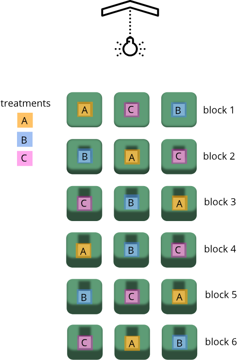
In this example, there are three different treatments (A, B, and C). The number of rows (or blocks) will be set to the number of replicates. Since we are interested in how light exposure differs from top to bottom, we will want our blocks to convey that difference; hence blocks should correspond to rows in the rack as each row is believed to have a different amount of light exposure. It is not necessary that there be enough replicates so as to account for all combinations of the order of treatments, and there is no need for a replicate size greater than that which accounts for all combinations. In this example, we are using six replicates which happens to account for all possible combinations of the treatment groups.
The randomized block design controls a source of random variation (a random effect) which might otherwise confound the effect of a treatment, and is of no interest. This design will have one or more treatments (fixed effects) which are of interest. The design is used to increase power by controlling variation from random effects, such as shelf height or illumination. It is also useful for breaking the experiment up into smaller, more convenient mini-experiments.
Latin Square Design
Latin square designs are unique in that they allow for (and require) two blocking factors. These designs are used to simultaneously control (or eliminate) two sources of nuisance variability while addressing the effect of (or variability caused by) one factor of interest. For a Latin square design to be created, each of the two blocking factors must have the same number of levels, and that number of levels must also be equal to the number of treatment (or factor of interest) levels.
For example, a Latin square design can be used if there was a study on the effect of five treatments that was done on five different days by five different technicians.
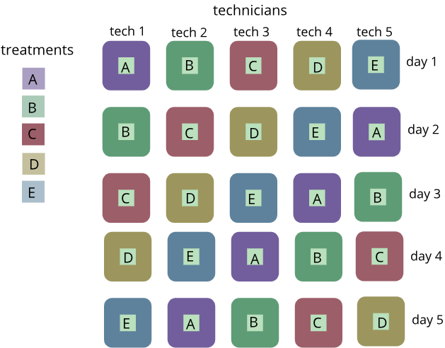
The blocks in this example would be technician (column) and day (row). The five different treatments (the factor of interest) are denoted by the letters A-E. We can remove the variation from our measured response to treatment in both directions if we consider both rows (day) and columns (technician) as factors in our design.
The Latin Square Design gets its name from the fact that we can write it as a square with Latin letters to correspond to the treatments. The treatment factor levels are the Latin letters in the Latin square design. The number of rows and columns has to correspond to the number of treatment levels. So, if we have five treatments then we would need to have five rows and five columns in order to create a Latin square. This gives us a design where we have each of the treatments and in each row and in each column.
Exercise 2: True or false?
- A completely randomized design can have different numbers in each treatment group.
- Completely randomized designs tolerate environmental changes, such as lighting differences, over time or space.
- A randomized block design ensures that the environment is the same for each experimental unit.
- A randomized block design can be used when experimental units are heterogeneous in age or weight.
Solution to Exercise 2
1). True. Numbers in each treatment group can differ, though sensitivity (true positive rate) could suffer.
2).
3).
4).
Exercise 3: Random assignment to diet
Use this subset of data containing 20 males and 20 females and their baseline body weights to randomize to two different diets: high fat and regular chow.
subset <- dat[dat$Sample[c(51:70, 475:494)],c("Sample", "Sex", "BW.3")]
1). Perform a complete randomization.
2). Perform a balanced randomization.
3). Check the sex ratio and difference in body weights.
4). Share the mean body weight for each group on the course etherpad.Solution to Exercise 3
This requires generation of random numbers. If diets are assigned in order, sample ID will be confounded with body weight if consecutive ID numbers were handled somehow by the same person or in the same way. 1). 2). 3). 4).
Key Points
Good experimental design minimizes error in a study.
Well-designed experiments are randomized, have adequate replicates, and feature local control of environmental variables.
There are three types of error in experiments: systematic, biological, and random.