Power calculation and sample size

Overview

Teaching: 0 min
Exercises: 0 min

Questions

• What role does the p-value (alpha) have in determining sample size for a study?

• What is type 2 error, and how does it correspond to the p-value and power of a test?

• What factors should be considered when estimating sample size for a study?

Objectives

• Calculate a sample size or power for a study that will be analyzed using a one fixed factor linear regression model.

Statistical power analysis is critical in experimental design. Before doing an experiment, it is important to calculate statistical power to estimate the sample size needed to detect an effect of a certain size with a specific degree of confidence. Underpowered studies are extremely common, which has led one of the most-cited scientists in medicine to claim that most published research findings are false.

Introduction

We’ll explore power calculations using the effects of two different diets on the body weights of mice. First we’ll load the data file.

# All code and text below is adapted from Irizarry & Love.
# http://genomicsclass.github.io/book/pages/power_calculations.html
# Exercises
# http://genomicsclass.github.io/book/pages/power_calculations_exercises.html

library(downloader)
url <- "https://raw.githubusercontent.com/smcclatchy/dals-inference/gh-pages/data/bodyWeights.csv"
filename <- "bodyWeights.csv"
if(!file.exists(filename)) download(url, destfile=filename)

# Read in DO850 body weight data.
dat <- read.csv("bodyWeights.csv") 

Now we’ll select body weight at 21 weeks for male mice on either a standard chow or high fat diet. We’ll examine the difference in mean body weight between males on high fat and those on a chow diet.

library(dplyr)

controlPopulation <- filter(dat, Sex == "M" & Diet == "chow") %>%  
  select(BW.21) %>% unlist

hfPopulation <- filter(dat, Sex == "M" & Diet == "hf") %>%  
  select(BW.21) %>% unlist

mu_hf <- mean(hfPopulation, na.rm = TRUE)
mu_control <- mean(controlPopulation, na.rm = TRUE)
print(mu_hf - mu_control)

[1] 6.696912

print((mu_hf - mu_control)/mu_control * 100) # percent increase

[1] 18.59599

What is the difference between body weight averages on a high fat vs. standard chow diet?

print(mu_hf - mu_control)

[1] 6.696912

What is the percentage increase in body weight of animals on high fat diet?

print((mu_hf - mu_control)/mu_control * 100) # percent increase

[1] 18.59599

Since we have access to the population, we know that in fact there is a substantial difference (greater than 0 between the average weights of the two male populations at 21 weeks of age.

We can see that, in some cases, when we take a sample and perform a t-test, we don’t always get a p-value smaller than 0.05. For example, here is a case where we take a sample of 3 mice and don’t achieve statistical significance at the 0.05 level:

set.seed(1)
N <- 3
hf <- sample(hfPopulation, N)
control <- sample(controlPopulation, N)
t.test(hf, control)$p.value

[1] 0.006750713

Did we make a mistake? By not rejecting the null hypothesis, are we saying the diet has no effect? The answer to this question is no. All we can say is that we did not reject the null hypothesis. But this does not necessarily imply that the null is true. The problem is that, in this particular instance, we don’t have enough power, a term we are now going to define. If you are doing scientific research, it is very likely that you will have to do a power calculation at some point. In many cases, it is an ethical obligation as it can help you avoid sacrificing mice unnecessarily or limiting the number of human subjects exposed to potential risk in a study. Here we explain what statistical power means.

Types of Error

Whenever we perform a statistical test, we are aware that we may make a mistake. This is why our p-values are not 0. Under the null, there is always a positive, perhaps very small, but still positive chance that we will reject the null when it is true. If the p-value is 0.05, it will happen 1 out of 20 times. This error is called type I error by statisticians.

A type I error is defined as rejecting the null when we should not. This is also referred to as a false positive. So why do we then use 0.05? Shouldn’t we use 0.000001 to be really sure? The reason we don’t use infinitesimal cut-offs to avoid type I errors at all cost is that there is another error we can commit: to not reject the null when we should. This is called a type II error or a false negative. The R code analysis above shows an example of a false negative: we did not reject the null hypothesis (at the 0.05 level) and, because we happen to know and peeked at the true population means, we know there is in fact a difference. Had we used a p-value cutoff of 0.25, we would not have made this mistake. However, in general, are we comfortable with a type I error rate of 1 in 4? Usually we are not.

The 0.05 and 0.01 Cut-offs Are Arbitrary

Most journals and regulatory agencies frequently insist that results be significant at the 0.01 or 0.05 levels. Of course there is nothing special about these numbers other than the fact that some of the first papers on p-values used these values as examples. Part of the goal of this book is to give readers a good understanding of what p-values and confidence intervals are so that these choices can be judged in an informed way. Unfortunately, in science, these cut-offs are applied somewhat mindlessly, but that topic is part of a complicated debate.

Power Calculation

Power is the probability of rejecting the null when the null is false. Of course “when the null is false” is a complicated statement because it can be false in many ways. $\Delta \equiv \mu_Y - \mu_X$ could be anything and the power actually depends on this parameter. It also depends on the standard error of your estimates which in turn depends on the sample size and the population standard deviations. In practice, we don’t know these so we usually report power for several plausible values of $\Delta$, $\sigma_X$, $\sigma_Y$ and various sample sizes. Statistical theory gives us formulas to calculate power. The pwr package performs these calculations for you. Here we will illustrate the concepts behind power by coding up simulations in R.

Suppose our sample size is:

N <- 4

and we will reject the null hypothesis at:

alpha <- 0.05

What is our power with this particular data? We will compute this probability by re-running the exercise many times and calculating the proportion of times the null hypothesis is rejected. Specifically, we will run:

B <- 2000

simulations. The simulation is as follows: we take a sample of size $N$ from both control and treatment groups, we perform a t-test comparing these two, and report if the p-value is less than alpha or not. We write a function that does this:

reject <- function(N, alpha=0.05){
   hf <- sample(hfPopulation, N) 
   control <- sample(controlPopulation, N)
   pval <- t.test(hf, control)$p.value
   pval < alpha
}

Here is an example of one simulation for a sample size of 12. The call to reject answers the question “Did we reject?”

reject(N)

[1] FALSE

Now we can use the replicate function to do this B times.

B <- 10
rejections <- replicate(B, reject(N))

Our power is just the proportion of times we correctly reject. So with $N=12$ our power is only:

mean(rejections)

[1] 0.1

This explains why the t-test was not rejecting when we knew the null was false. With a sample size of just 12, our power is about 0.1 percent. To guard against false positives at the 0.05 level, we had set the threshold at a high enough level that resulted in many type II errors.

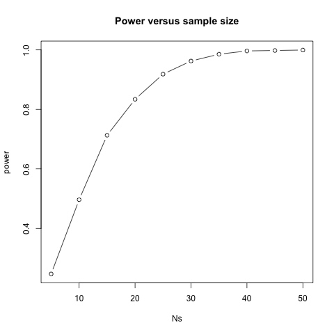
Let’s see how power improves with N. We will use the function sapply, which applies a function to each of the elements of a vector. We want to repeat the above for the following sample sizes from 5 to 50 in increments of 5:

Ns <- seq(from = 5, to = 50, by = 5)

So we use apply like this:

power <- sapply(Ns, function(N){
  rejections <- replicate(B, reject(N))
  mean(rejections)
  })

For each of the three simulations, the above code returns the proportion of times we reject. Not surprisingly power increases with N:

plot(Ns, power, type="b")

Similarly, if we change the level alpha at which we reject, power changes. The smaller I want the chance of type I error to be, the less power I will have. Another way of saying this is that we trade off between the two types of error. We can see this by writing similar code, but keeping $N$ fixed and considering several values of alpha:

N <- 30
alphas <- c(0.1, 0.05, 0.01, 0.001, 0.0001)
power <- sapply(alphas, function(alpha){
  rejections <- replicate(B, reject(N, alpha=alpha))
  mean(rejections)
})
plot(alphas, power, xlab="alpha", type="b", log="x")

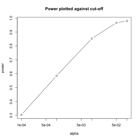
Note that the x-axis in this last plot is in the log scale.

There is no “right” power or “right” alpha level, but it is important that you understand what each means.

To see this clearly, you could create a plot with curves of power versus N. Show several curves in the same plot with color representing alpha level.

p-values Are Arbitrary under the Alternative Hypothesis

Another consequence of what we have learned about power is that p-values are somewhat arbitrary when the null hypothesis is not true and therefore the alternative hypothesis is true (the difference between the population means is not zero). When the alternative hypothesis is true, we can make a p-value as small as we want simply by increasing the sample size (supposing that we have an infinite population to sample from). We can show this property of p-values by drawing larger and larger samples from our population and calculating p-values. This works because, in our case, we know that the alternative hypothesis is true, since we have access to the populations and can calculate the difference in their means.

First write a function that returns a p-value for a given sample size $N$:

calculatePvalue <- function(N) {
   hf <- sample(hfPopulation, N) 
   control <- sample(controlPopulation, N)
   t.test(hf, control)$p.value
}

We have a limit here of 197 for the high-fat diet population, but we can see the effect well before we get to 197. For each sample size, we will calculate a few p-values. We can do this by repeating each value of $N$ a few times.

Ns <- seq(from = 10, to = length(hfPopulation), by=10)
Ns_rep <- rep(Ns, each=10)

Again we use sapply to run our simulations:

pvalues <- sapply(Ns_rep, calculatePvalue)

Now we can plot the 10 p-values we generated for each sample size:

plot(Ns_rep, pvalues, log="y", xlab="sample size",
     ylab="p-values")
abline(h=c(.01, .05), col="red", lwd=2)

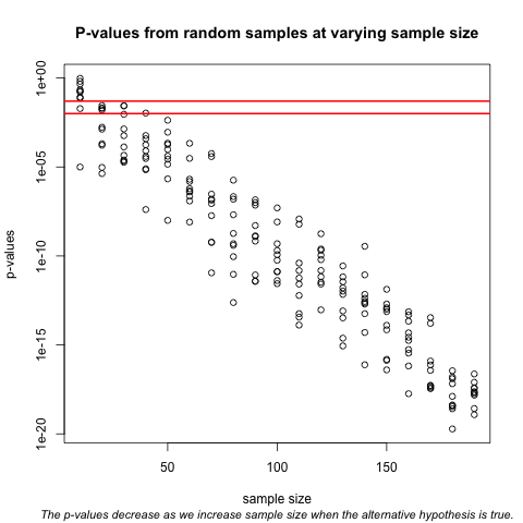
Note that the y-axis is log scale and that the p-values show a decreasing trend all the way to $10^{-8}$ as the sample size gets larger. The standard cutoffs of 0.01 and 0.05 are indicated with horizontal red lines.

It is important to remember that p-values are not more interesting as they become very very small. Once we have convinced ourselves to reject the null hypothesis at a threshold we find reasonable, having an even smaller p-value just means that we sampled more mice than was necessary. Having a larger sample size does help to increase the precision of our estimate of the difference $\Delta$, but the fact that the p-value becomes very very small is just a natural consequence of the mathematics of the test. The p-values get smaller and smaller with increasing sample size because the numerator of the t-statistic has $\sqrt{N}$ (for equal sized groups, and a similar effect occurs when $M \neq N$). Therefore, if $\Delta$ is non-zero, the t-statistic will increase with $N$.

Therefore, a better statistic to report is the effect size with a confidence interval or some statistic which gives the reader a sense of the change in a meaningful scale. We can report the effect size as a percent by dividing the difference and the confidence interval by the control population mean:

N <- 12
hf <- sample(hfPopulation, N)
control <- sample(controlPopulation, N)
diff <- mean(hf, na.rm = TRUE) - mean(control, na.rm = TRUE)
diff / mean(control, na.rm = TRUE) * 100

[1] 24.24669

t.test(hf, control)$conf.int / mean(control, na.rm = TRUE) * 100

[1]  5.940412 42.552963
attr(,"conf.level")
[1] 0.95

In addition, we can report a statistic called Cohen’s d, which is the difference between the groups divided by the pooled standard deviation of the two groups.

sd_pool <- sqrt(((N - 1) * var(hf, na.rm = TRUE) + (N - 1) * var(control, na.rm = TRUE))/(2 * N - 2))
diff / sd_pool

[1] 1.145321

This tells us how many standard deviations of the data the mean of the high-fat diet group is from the control group. Under the alternative hypothesis, unlike the t-statistic which is guaranteed to increase, the effect size and Cohen’s d will become more precise.

Challenge 1: Power and sample size calculation for two treatment comparison (Gary’s suggestion)

1). Specify power and size of test, variance, meaningful difference. Compute N.
2). Specify N, power, variance. Compute meaningful difference (what can I hope to get with my budget fixed?).

Solution to Challenge 1

Challenge 2: Draw some power curves (Gary’s suggestion)

1). How are they affected by alpha, beta, delta, N? 2). If you double the sample size how does delta change? Use formulas, functions, statistical rules of thumb. Share your power curve with your neighbor. How would you choose sample size? What do you consider wasteful sample sizes when looking at these curves?

Solution to Challenge 2

Challenge 3: Compute power by simulation (Gary’s suggestion)

Learn how to simulate data. Draw power curves from simulations. Compare to theoretical curves.

Solution to Challenge 3

Challenge 4 (advanced): Permutation tests (Gary’s suggestion)

Solution to Challenge 4

Challenge 5: Watch A Biologist Talks to a Statistician

Do you empathize more now with the biologist or with the statistician?

Key Points

• When designing an experiment, use biological replicates.

• Choose a single representative value (the mean, median, or mode) for technical replicates.