Cross-validation

Overview

Teaching: 30 min
Exercises: 30 min

Questions

How can the best configuration of parameters be selected for a machine learning model using only the data available?

Objectives

Create a set of fold indices for cross-validation

Select the best configuration for a machine learning model using cross-validation

Cross-validation

Here we describe cross-validation: one of the fundamental methods in machine learning for method assessment and picking parameters in a prediction or machine learning task. Suppose we have a set of observations with many features and each observation is associated with a label. We will call this set our training data. Our task is to predict the label of any new samples by learning patterns from the training data. For a concrete example, let’s consider gene expression values, where each gene acts as a feature. We will be given a new set of unlabeled data (the test data) with the task of predicting the tissue type of the new samples.

If we choose a machine learning algorithm with a tunable parameter, we have to come up with a strategy for picking an optimal value for this parameter. We could try some values, and then just choose the one which performs the best on our training data, in terms of the number of errors the algorithm would make if we apply it to the samples we have been given for training. However, we have seen how this leads to over-fitting.

Let’s start by loading the tissue gene expression dataset:

library(tissuesGeneExpression)
data(tissuesGeneExpression)

For illustration purposes, we will drop one of the tissues which doesn’t have many samples:

table(tissue)

tissue
 cerebellum       colon endometrium hippocampus      kidney       liver 
         38          34          15          31          39          26 
   placenta 
          6 

ind <- which(tissue != "placenta")
y <- tissue[ind]
X <- t( e[,ind] )

This tissue will not form part of our example.

Now let’s try out k-nearest neighbors for classification, using $k=5$. What is our average error in predicting the tissue in the training set, when we’ve used the same data for training and for testing?

library(class)
pred <- knn(train =  X, test = X, cl=y, k=5)
mean(y != pred)

[1] 0

We have no errors in prediction in the training set with $k=5$. What if we use $k=1$?

pred <- knn(train=X, test=X, cl=y, k=1)
mean(y != pred)

[1] 0

Trying to classify the same observations as we use to train the model can be very misleading. In fact, for k-nearest neighbors, using k=1 will always give 0 classification error in the training set, because we use the single observation to classify itself. The reliable way to get a sense of the performance of an algorithm is to make it give a prediction for a sample it has never seen. Similarly, if we want to know what the best value for a tunable parameter is, we need to see how different values of the parameter perform on samples, which are not in the training data.

Cross-validation is a widely-used method in machine learning, which solves this training and test data problem, while still using all the data for testing the predictive accuracy. It accomplishes this by splitting the data into a number of folds. If we have $N$ folds, then the first step of the algorithm is to train the algorithm using $(N-1)$ of the folds, and test the algorithm’s accuracy on the single left-out fold. This is then repeated N times until each fold has been used as in the test set. If we have $M$ parameter settings to try out, then this is accomplished in an outer loop, so we have to fit the algorithm a total of $N \times M$ times.

We will use the createFolds function from the caret package to make 5 folds of our gene expression data, which are balanced over the tissues. Don’t be confused by the fact that the createFolds function uses the same letter ‘k’ as the ‘k’ in k-nearest neighbors. These ‘k’ are totally unrelated. The caret function createFolds is asking for how many folds to create, the $N$ from above. The ‘k’ in the knn function is for how many closest observations to use in classifying a new sample. Here we will create 10 folds:

library(caret)
set.seed(1)
idx <- createFolds(y, k=10)
sapply(idx, length)

Fold01 Fold02 Fold03 Fold04 Fold05 Fold06 Fold07 Fold08 Fold09 Fold10 
    19     19     18     18     19     18     20     16     16     20 

The folds are returned as a list of numeric indices. The first fold of data is therefore:

y[idx[[1]]] ##the labels

 [1] "kidney"      "hippocampus" "hippocampus" "hippocampus" "cerebellum" 
 [6] "cerebellum"  "cerebellum"  "kidney"      "kidney"      "kidney"     
[11] "colon"       "colon"       "colon"       "liver"       "endometrium"
[16] "endometrium" "liver"       "liver"       "cerebellum" 

head( X[idx[[1]], 1:3] ) ##the genes (only showing the first 3 genes...)

                1007_s_at  1053_at   117_at
GSM12105.CEL.gz  9.913031 6.337478 7.983850
GSM21209.cel.gz 11.667431 5.785190 7.666343
GSM21215.cel.gz 10.361340 5.663634 7.328729
GSM21218.cel.gz 10.757734 5.984170 8.525524
GSM87066.cel.gz  9.746007 5.886079 7.459517
GSM87085.cel.gz  9.864295 5.753874 7.712646

We can see that, in fact, the tissues are fairly equally represented across the 10 folds:

sapply(idx, function(i) table(y[i]))

            Fold01 Fold02 Fold03 Fold04 Fold05 Fold06 Fold07 Fold08 Fold09
cerebellum       4      4      4      4      4      3      4      3      4
colon            3      4      4      3      3      3      4      3      3
endometrium      2      1      1      1      2      2      2      1      1
hippocampus      3      3      3      3      3      3      3      3      3
kidney           4      4      4      4      4      4      4      4      3
liver            3      3      2      3      3      3      3      2      2
            Fold10
cerebellum       4
colon            4
endometrium      2
hippocampus      4
kidney           4
liver            2

Because tissues have very different gene expression profiles, predicting tissue with all genes will be very easy. For illustration purposes we will try to predict tissue type with just two dimensional data. We will reduce the dimension of our data using cmdscale:

library(rafalib)
mypar()
Xsmall <- cmdscale(dist(X))
plot(Xsmall,col=as.fumeric(y))
legend("topleft",levels(factor(y)),fill=seq_along(levels(factor(y))))

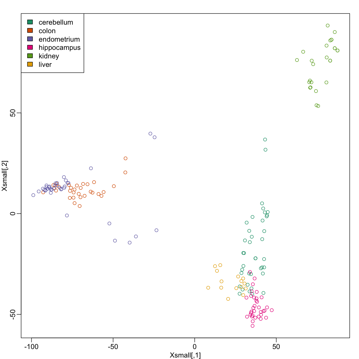
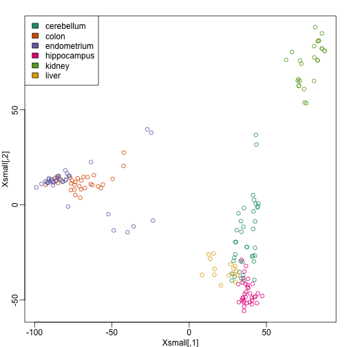
First two PCs of the tissue gene expression data with color representing tissue. We use these two PCs as our two predictors throughout.

Now we can try out the k-nearest neighbors method on a single fold. We provide the knn function with all the samples in Xsmall except those which are in the first fold. We remove these samples using the code -idx[[1]] inside the square brackets. We then use those samples in the test set. The cl argument is for the true classifications or labels (here, tissue) of the training data. We use 5 observations to classify in our k-nearest neighbor algorithm:

pred <- knn(train=Xsmall[ -idx[[1]] , ], test=Xsmall[ idx[[1]], ], cl=y[ -idx[[1]] ], k=5)
table(true=y[ idx[[1]] ], pred)

             pred
true          cerebellum colon endometrium hippocampus kidney liver
  cerebellum           4     0           0           0      0     0
  colon                0     2           0           0      1     0
  endometrium          0     0           2           0      0     0
  hippocampus          2     0           0           1      0     0
  kidney               0     0           0           0      4     0
  liver                0     0           0           0      0     3

mean(y[ idx[[1]] ] != pred)

[1] 0.1578947

Now we have some misclassifications. How well do we do for the rest of the folds?

for (i in 1:10) {
  pred <- knn(train=Xsmall[ -idx[[i]] , ], test=Xsmall[ idx[[i]], ], cl=y[ -idx[[i]] ], k=5)
  print(paste0(i,") error rate: ", round(mean(y[ idx[[i]] ] != pred),3)))
}

[1] "1) error rate: 0.158"
[1] "2) error rate: 0.158"
[1] "3) error rate: 0.278"
[1] "4) error rate: 0.167"
[1] "5) error rate: 0.158"
[1] "6) error rate: 0.167"
[1] "7) error rate: 0.25"
[1] "8) error rate: 0.188"
[1] "9) error rate: 0.062"
[1] "10) error rate: 0.1"

So we can see there is some variation for each fold, with error rates hovering around 0.1-0.3. But is k=5 the best setting for the k parameter? In order to explore the best setting for k, we need to create an outer loop, where we try different values for k, and then calculate the average test set error across all the folds.

We will try out each value of k from 1 to 12. Instead of using two for loops, we will use sapply:

set.seed(1)
ks <- 1:12
res <- sapply(ks, function(k) {
  ##try out each version of k from 1 to 12
  res.k <- sapply(seq_along(idx), function(i) {
    ##loop over each of the 10 cross-validation folds
    ##predict the held-out samples using k nearest neighbors
    pred <- knn(train=Xsmall[ -idx[[i]], ],
                test=Xsmall[ idx[[i]], ],
                cl=y[ -idx[[i]] ], k = k)
    ##the ratio of misclassified samples
    mean(y[ idx[[i]] ] != pred)
  })
  ##average over the 10 folds
  mean(res.k)
})

Now for each value of k, we have an associated test set error rate from the cross-validation procedure.

res

 [1] 0.1882164 0.1692032 0.1694664 0.1639108 0.1511184 0.1586184 0.1589108
 [8] 0.1865058 0.1880482 0.1714108 0.1759795 0.1744664

We can then plot the error rate for each value of k, which helps us to see in what region there might be a minimal error rate:

plot(ks, res, type="o",ylab="misclassification error")

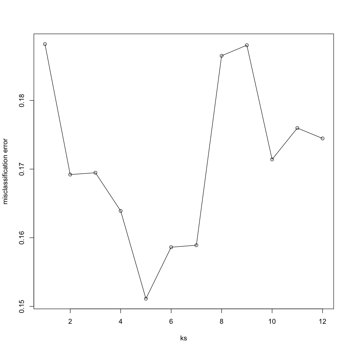
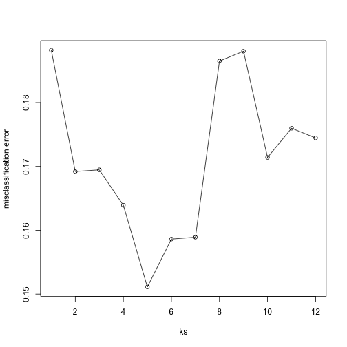
Misclassification error versus number of neighbors.

Remember, because the training set is a random sample and because our fold-generation procedure involves random number generation, the “best” value of k we pick through this procedure is also a random variable. If we had new training data and if we recreated our folds, we might get a different value for the optimal k.

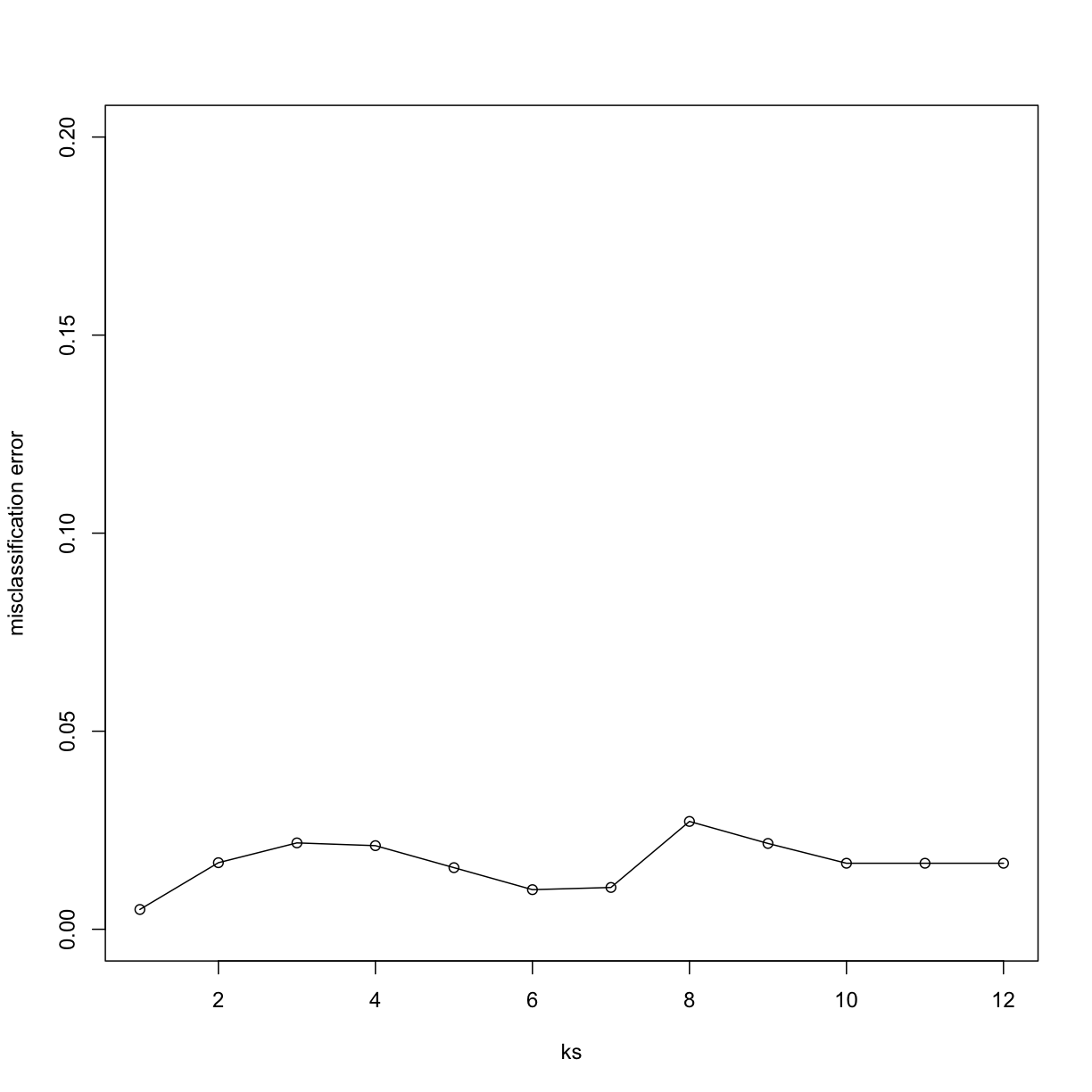
Finally, to show that gene expression can perfectly predict tissue, we use 5 dimensions instead of 2, which results in perfect prediction:

Xsmall <- cmdscale(dist(X),k=5)
set.seed(1)
ks <- 1:12
res <- sapply(ks, function(k) {
  res.k <- sapply(seq_along(idx), function(i) {
    pred <- knn(train=Xsmall[ -idx[[i]], ],
                test=Xsmall[ idx[[i]], ],
                cl=y[ -idx[[i]] ], k = k)
    mean(y[ idx[[i]] ] != pred)
  })
  mean(res.k)
})
plot(ks, res, type="o",ylim=c(0,0.20),ylab="misclassification error")

Misclassification error versus number of neighbors when we use 5 dimensions instead of 2.

Important note: we applied cmdscale to the entire dataset to create a smaller one for illustration purposes. However, in a real machine learning application, this may result in an underestimation of test set error for small sample sizes, where dimension reduction using the unlabeled full dataset gives a boost in performance. A safer choice would have been to transform the data separately for each fold, by calculating a rotation and dimension reduction using the training set only and applying this to the test set.

Exercises

Load the following dataset:

library(GSE5859Subset)
data(GSE5859Subset)

And define the outcome and predictors. To make the problem more difficult, we will only consider autosomal genes:

y = factor(sampleInfo$group)
X = t(geneExpression)
out = which(geneAnnotation$CHR %in% c("chrX","chrY"))
X = X[,-out]

Exercise 1

Use the createFold function in the caret package, set the seed to 1 set.seed(1) and create 10 folds of y. What is the 2nd entry in the fold 3?
Solution
library(caret)
set.seed(1)
idx <- createFolds(y, k = 10)
# Select the set of indices corresponding to the third fold
# using idx[[3]], then print the second index of that fold
idx[[3]][2]

Exercise 2

We are going to use kNN. We are going to consider a smaller set of predictors by using filtering gene using t-tests. Specifically, we will perform a t-test and select the $m$ genes with the smallest p-values.

Let m = 8 and k = 5 and train kNN by leaving out the second fold idx[[2]]. How many mistakes do we make on the test set? Remember it is indispensable that you perform the t-test on the training data. Use all 10 folds, keep k = 5. Hint: be careful about indexing.
Solution
library(genefilter)
m <- 8 # number of genes

# `rowttests` performs a t-test on the expression of each gene
pvals <- rowttests(t(X[-idx[[2]],]),y[-idx[[2]]])$p.value

# We use the p-value to identify the genes that present a
# significant effect (i.e. the effect is statistically
# different from 0). That is achieved by ordering `pvals`
# in increasing order, and taking the `m` smallest p-values
ind <- order(pvals)[1:m]

# Then the k-nearest-neighbor algorithm is executed only
# considering these `m` most significant genes.
pred <- knn(train = X[-idx[[2]],ind],
            test = X[idx[[2]],ind],
            cl = y[-idx[[2]]], k = 5)

# This command computes the total number of examples that
# were miss-classified by the knn algorithm.
sum(pred != y[idx[[2]]])

Exercise 3

Now run through all 5 folds. What is our error rate? (total number of errors / total predictions)

Solution

# Now run the previous piece of code for each fold
n_fold <- length(idx)
res <- vector('double', n_fold)
m <- 8
for (i in seq(n_fold)) {
  # To be fair and only use the information we have at the moment
  # of training, we perform the t-tests only on the training set.
  pvals <- rowttests(t(X[-idx[[i]],]),y[-idx[[i]]])$p.value
  ind <- order(pvals)[1:m]
  # We will use again the top m=8 genes that showed the most
  # significant effect according to the previous t-tests.
  pred <- knn(train = X[-idx[[i]],ind],
              test = X[idx[[i]],ind],
              cl = y[-idx[[i]]], k = 5)
  res[[i]] <- sum(pred != y[idx[[i]]])
}
# Compute the average performance of the knn algorithm achieved on
# the ten folds.
sum(res)/length(y)

Exercise 4

Now we are going to select the best values of k and m. Use the expand grid function to try out the following values:

ms = 2^c(1:11)
ks = seq(1,9,2)
# Compute all possible pairs of configurations of number of most
# significant genes and number of neighbors for the knn algorithm.
params = expand.grid(k=ks, m=ms)

Now use apply or a for-loop to obtain error rates for each of these pairs of parameters. Which pair of parameters minimizes the error rate?

Solution

n_fold <- length(idx)
# Store the mean performance on the ten folds of the knn algorithm
# using each pair of parameters.
error_rate_avg = vector('double',nrow(params))
# Iterate over each pair of parameters:
# (number of neighbors, number of genes)
for (j in seq(nrow(params))) {
    # Iterate over each fold
    for (i in seq(n_fold)) {
        # Again perform the t-tests only on the training set
        pvals <- rowttests(t(X[-idx[[i]],]),y[-idx[[i]]])$p.value
        # This time we take the top number of genes given by
        # the current pair of parameters `param[j,][[2]]`
        ind <- order(pvals)[1:params[j,][[2]]]

        # Train the knn algorithm using the train set, and
        # evaluating on the test set of the current fold `idx[[i]]`.
        # The knn is trained using the number of neighbors given
        # by the current pair of parameters `param[j,][[1]]`
        pred <- knn(train = X[-idx[[i]],ind],
                    test = X[idx[[i]],ind],
                    cl = y[-idx[[i]]],
                    k = params[j,][[1]])
        res[[i]] <- sum(pred != y[idx[[i]]])
    }
    # Approximate how our knn algorithm would perform with unseen data
    # by computing the mean error achieved on all the folds.
    error_rate_avg[[j]] <- sum(res)/length(y)
}
# Find the pair of parameters (number of neighbors, number of genes)
# that achieves the lowest expected error.
ind <- which(error_rate_avg == min(error_rate_avg))

# Print that pair of parameters and the corresponding error rate
# achieved
params[ind,] # answer
min(error_rate_avg) # minimum error rate

Exercise 5

Repeat exercise 4, but now perform the t-test filtering before the cross validation. Note how this biases the entire result and gives us much lower estimated error rates.

Solution

# We perform the same experiment with the exception that
# this time we perform the t-tests on all the dataset to
# choose the top number of genes with most significant
# effect.
ms = 2^c(1:11)
ks = seq(1,9,2)
params = expand.grid(k=ks, m=ms)
n_fold <- length(idx)
error_rate_avg = vector('double',nrow(params))
for (j in seq(nrow(params))) {
    for (i in seq(n_fold)) {
        # Here we use the complete dataset to select the genes,
        # rather than only the examples corresponding to this fold.
        pvals <- rowttests(t(X),y)$p.value
        ind <- order(pvals)[1:params[j,][[2]]]
        pred <- knn(train = X[-idx[[i]],ind],
                    test = X[idx[[i]],ind],
                    cl = y[-idx[[i]]], k = params[j,][[1]])
        res[[i]] <- sum(pred != y[idx[[i]]])
    }
    error_rate_avg[[j]] <- sum(res)/length(y)
}
min(error_rate_avg) # minimum error rate
mean(error_rate_avg) # mean error rate

The error rate is much lower than the one in Exercise 4 because we did not filter out p values from the test data in this case. This is not a correct practice. The practice shown in Exercise 4 is correct.

Exercise 6

Repeat exercise 3, but now, instead of sampleInfo$group, use y = factor(as.numeric(format( sampleInfo$date, "%m")=="06")) What is the minimum error rate now? We achieve much lower error rates when predicting date than when predicting the group. Because group is confounded with date, it is very possible that these predictors have no information about group and that our lower 0.5 error rates are due to the confounding with date. We will learn more about this in the batch effect chapter.
Solution
# We use 'y' as the date the sample was taken as class.
# However, notice that this is introducing a `batch effect`.
y = factor(as.numeric(format( sampleInfo$date, "%m")=="06"))

ms = 2^c(1:11)
ks = seq(1,9,2)
params = expand.grid(k=ks, m=ms)
n_fold <- length(idx)
error_rate_avg = vector('double',nrow(params))
for (j in seq(nrow(params))) {
    for (i in seq(n_fold)) {
        pvals <- rowttests(t(X[-idx[[i]],]),y[-idx[[i]]])$p.value
        ind <- order(pvals)[1:params[j,][[2]]]
        pred <- knn(train = X[-idx[[i]],ind],
                    test = X[idx[[i]],ind],
                    cl = y[-idx[[i]]], k = params[j,][[1]])
        res[[i]] <- sum(pred != y[idx[[i]]])
    }
    error_rate_avg[[j]] <- sum(res)/length(y)
}
min(error_rate_avg) # minimum error rate
mean(error_rate_avg) # mean error rate

Key Points

The mean validation error obtained from cross-validation is a better approximation of the test error (real world data) than the training error iteself

previous episode

Machine Learning for Biomedical Science

lesson home

Cross-validation

Overview