Data and Study Design
Last updated on 2025-10-07 | Edit this page
Overview
Questions
- Which data will we explore in this course?
- How was the study that generated the data designed?
- What are some critical design elements for rigorous, reproducible spatial transcriptomics experiments?
Objectives
- Describe a spatial transcriptomics experiment.
- Identify important elements for good experimental design.
The Data
Recall that tissue is laid on a glass slide containing spots with primers to capture mRNA. The graphic below details a Visium slide with four capture areas. Each capture area has arrays of barcoded spots containing oligonucleotides. The oligonucleotides each contain a poly(dT) sequence for capture of polyadenylated molecules, a unique molecular identifier (UMI) to identify duplicate molecules, a spatial barcode shared by all oligonucleotides within the same spot, and a partial read for library preparation and sequencing.
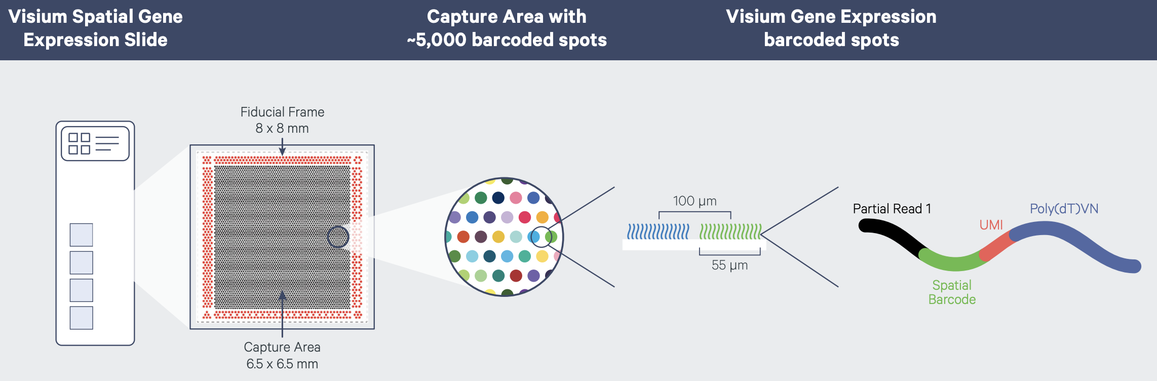
In spatial transcriptomics the barcode indicates the x-y coordinates of the spot. Barcodes are generic identifiers that identify different things in different technologies. A barcode in single-cell transcriptomics, for example, refers to a single cell, not to a spot on a slide. When you see barcodes in ST data, think spot, not single cell. In fact, one spot can capture mRNA from many cells. This is a feature of ST experiments that is distinct from single-cell transcriptomics experiments. As a result, many single-cell methods won’t work with ST data. Later we will look at methods to deconvolve cell types per spot to determine the number and types of cells in each spot. Spots can contain zero, one, or many cells.
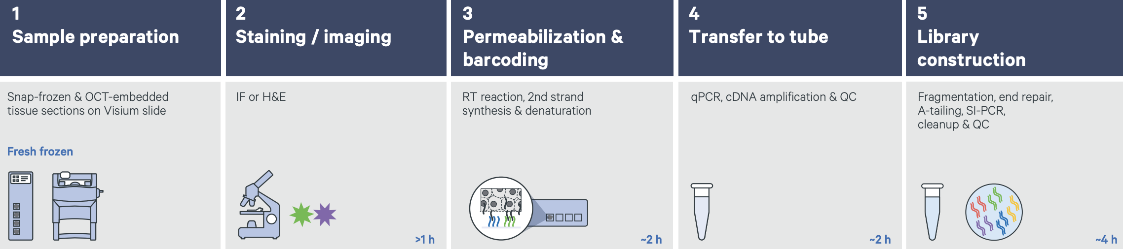
The graphic below shows a Visium workflow for fresh-frozen tissues.
 Graphic from
Grant
application resources for Visium products at 10X Genomics
Graphic from
Grant
application resources for Visium products at 10X Genomics
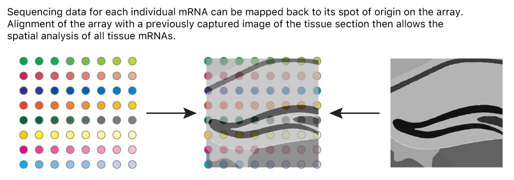
Count data for each mRNA are mapped back to spots on the slide to indicate the tissue position of gene expression. An image of the tissue overlaid on the array of spots pinpoints spatial gene expression in the tissue.
Adapted from James Chell, Spatial transcriptomics ii, CC BY-SA 4.0
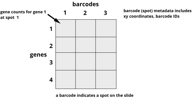
Data from the 10X Genomics Visium platform contain gene identifiers in rows and barcode identifiers in columns. In the graphic below, row 1 of column 1 contains the mRNA counts for gene 1 at barcode (spot) 1.
Challenge 1: Row and column sums
What does the sum of a single row signify?
What does the sum of a single column signify?
The row sum is the total expression of one gene across all spots on the slide.
R
sum('data[1, ]')
The column sum is the total expression of all genes for one spot on the slide.
R
sum('data[ , 1]')
Design and Motivation of Prefrontal Cortex Study
We will use data from a study of the human prefrontal cortex published in Transcriptome-scale spatial gene expression in the human dorsolateral prefrontal cortex by Maynard et al, Nat Neurosci 24, 425–436 (2021). This region of the brain, involved in higher-order cognition and managing thoughts and actions in conformance with internal goals, is particularly amenable to spatial analyses because its structure is intimately tied to its function. Specifically, the six cortical layers and the white matter shown below are comprised of cells with distinct gene expression profiles and differing patterns of morphology, physiology, and connectivity.
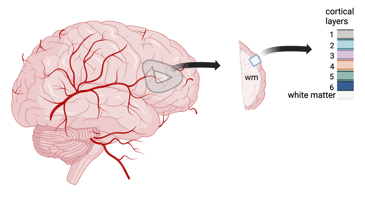
Adapted from Maynard et al, Nat Neurosci 24, 425–436 (2021). Created with BioRender.com.
The dorsolateral prefrontal cortex is implicated in some neuropsychiatric disorders such as autism spectrum disorder (ASD) and schizophrenia disorder (SCZD), and differences in gene expression and pathology are located in specific cortical layers. Localizing gene expression at cellular resolution within the six layers can illuminate disease mechanisms and brain development. As such, the authors aimed to map gene expression to the spatial organization of the six cortical layers. This course will largely follow their analyses in defining the gene expression markers of the cortical layers.
Spatial transcriptomics has several advantages relative to other technologies in meeting the authors’ objective. Owing to their large size and fragility, human neurons are difficult to isolate with scRNA-seq. This has motivated the use of single-nucleus(sn)RNA-seq in most studies. Unfortunately, this modality fails to capture cytoplasmic compartments of the cell, as well as axons and dendrites, and the genes within these regions have been associated with SCZD and ASD. Laser capture microdissection followed by sequencing does capture all cellular compartments, but can not be use to detect spatial gradients of gene expression since it removes tissues from their spatial context. Spatial transcriptomics offers the ability both to capture the entire repertoire of cells resident in the brain and to establish the expression gradient across them within the spatial context of the intact tissue.
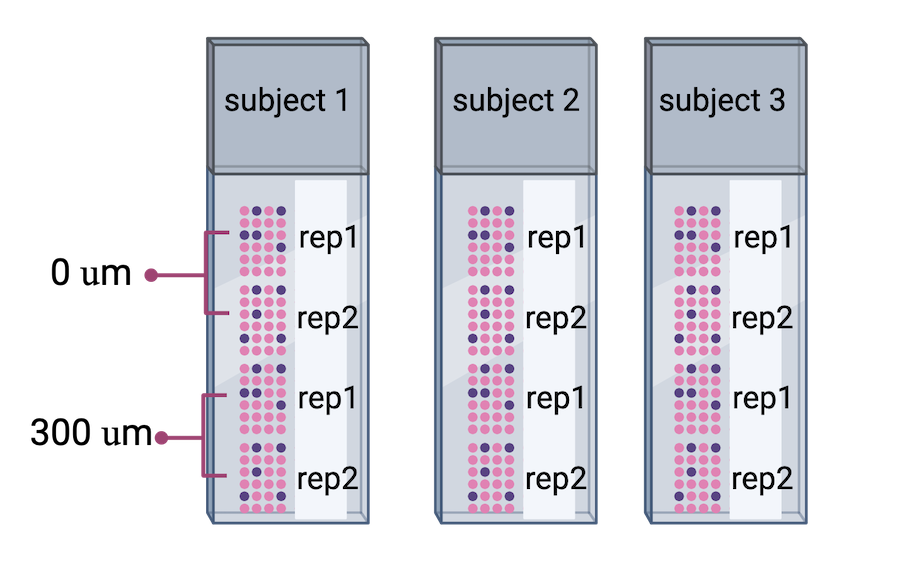
The authors proceeded in their spatial transcriptomics study by selecting wwo pairs of spatially adjacent replicates from three neurotypical donors. The second pair of replicates was taken from 300 microns posterior to the first pair of replicates.
 Adapted from
Maynard et al, Nat
Neurosci 24, 425–436 (2021).
Created with BioRender.com.
Adapted from
Maynard et al, Nat
Neurosci 24, 425–436 (2021).
Created with BioRender.com.
Challenge 2: What do you notice?
What do you notice about the experimental design that might create issues during data analysis? Why might the authors have done the experiment this way? Is there anything that can be done about this?
Human brain tissues start to deteriorate at death. Brain banks that provide tissue for studies requiring intact mRNA will quickly remove the brain and rapidly weigh, examine, dissect and freeze it to optimize mRNA integrity. For this study, dorsolateral prefrontal cortex samples were embedded in a medium (see Methods section) and then cryosectioned. Sections were then placed on chilled Visium slides, fixed and stained.
This whole process might have depended on donor availability. All three donors were neurotypical, and it’s not clear how they died (e.g., an accident, a terminal illness, old age) and how that might have impacted availability or mRNA quality. Suffice it to say that it might not have been possible to predict when samples would be available, so it might not have been possible to randomize the samples from each donor to different Visium slides.
Sometimes you might have to confound variables in your study due to sample availability or other factors. The key thing is to know that confounding has occurred.
Important considerations for rigorous, reproducible experiments
Good experimental design plays a critical role in obtaining reliable and meaningful results and is an essential feature of rigorous, reproducible experiments. Designed experiments aim to describe and explain variability under experimental conditions. Variability is natural in the real world. A medication given to a group of patients will affect each of them differently. A specific diet given to a cage of mice will affect each mouse differently. Ideally if something is measured many times, each measurement will give exactly the same result and will represent the true value. This ideal doesn’t exist in the real world. Variability is a feature of natural systems and also a natural part of every experiment we undertake.
Replication
To figure out whether a difference in responses is real or inherently random, replication applies the same treatment to multiple experimental units. The variability of the responses within a set of replicates provides a measure against which we can compare differences among different treatments. Experimental error describes the variability in the responses. Random variation (a.k.a random error or noise) reflects imprecision, but not inaccuracy. Larger sample sizes reduce this imprecision.
In addition to random (experimental) error, systematic error or bias occurs when there are deviations in measurements or observations that consistently either overestimate or underestimate the true value. As an example, a scale might be calibrated so that mass measurements are consistently too high or too low. Unlike random error, systematic error is consistent in one direction, is predictable and follows a pattern. Larger sample sizes don’t correct for systematic bias; equipment or measurement calibration does. Technical replicates define this systematic bias by running the same sample through the machine or measurement protocol multiple times to characterize the variation caused by equipment or protocols.
A biological replicate measures different biological samples in parallel to estimate the variation caused by the unique biology of the samples. The sample or group of samples are derived from the same biological source, such as cells, tissues, organisms, or individuals. Biological replicates assess the variability and reproducibility of experimental results. The greater the number of biological replicates, the greater the precision (the closeness of two or more measurements to each other). Having a large enough sample size to ensure high precision is necessary to ensure reproducible results. Note that increasing the number of technical replicates will not help to characterize biological variability! It is used to characterize systematic error, not experimental error.
Challenge 3: Which kind of error?
A study used to determine the effect of a drug on weight loss could
have the following sources of experimental error. Classify the following
sources as either biological, systematic, or random error.
1). A scale is broken and provides inconsistent readings.
2). A scale is calibrated wrongly and consistently measures mice 1 gram
heavier.
3). A mouse has an unusually high weight compared to its experimental
group (e.g., it is an outlier).
4). Strong atmospheric low pressure and accompanying storms affect
instrument readings, animal behavior, and indoor relative humidity.
1). random, because the scale is broken and provides any kind of
random reading it comes up with (inconsistent reading)
2). systematic
3). biological
4). random or systematic; you argue which and explain why
Challenge 4: How many technical and biological replicates?
In each scenario described below, identify how many technical and how many biological replicates are represented. What conclusions can be drawn about experimental error in each scenario?
1). One person is weighed on a scale five times.
2). Five people are weighed on a scale one time each.
3). Five people are weighed on a scale three times each.
4). A cell line is equally divided into four samples. Two samples
receive a drug treatment, and the other two samples receive a different
treatment. The response of each sample is measured three times to
produce twelve total observations. In addition to the number of
replicates, can you identify how many experimental units there
are?
5). A cell line is equally divided into two samples. One sample receives
a drug treatment, and the other sample receives a different treatment.
Each sample is then further divided into two subsamples, each of which
is measured three times to produce twelve total observations. In
addition to the number of replicates, can you identify how many
experimental units there are?
1). One biological sample (not replicated) with five technical
replicates. The only conclusion to be drawn from the measurements would
be better characterization of systematic error in measuring. It would
help to describe variation produced by the instrument itself, the scale.
The measurements would not generalize to other people.
2). Five biological replicates with one technical measurement (not
replicated). The conclusion would be a single snapshot of the weight of
each person, which would not capture systematic error or variation in
measurement of the scale. There are five biological replicates, which
would increase precision, however, there is considerable other variation
that is unaccounted for.
3). Five biological replicates with three technical replicates each. The
three technical replicates would help to characterize systematic error,
while the five biological replicates would help to characterize
biological variability.
4). Four biological replicates with three technical replicates each. The
three technical replicates would help to characterize systematic error,
while the four biological replicates would help to characterize
biological variability. Since the treatments are applied to each of the
four samples, there are four experimental units.
5). Two biological replicates with three technical replicates each.
Since the treatments are applied to only the two original samples, there
are only two experimental units.
Randomization
Randomization minimizes bias, moderates experimental error (a.k.a. noise), and ensures that our comparisons between treatment groups are valid. Randomized studies assign experimental units to treatment groups randomly by pulling a number out of a hat or using a computer’s random number generator. The main purpose for randomization comes later during statistical analysis, where we compare the data we have with the data distribution we might have obtained by random chance. Random assignment (allocation) of experimental units to treatment groups prevents the subjective bias that might be introduced by an experimenter who selects, even in good faith and with good intention, which experimental units should get which treatment.
Randomization also accounts for or cancels out effects of “nuisance” variables like the time or day of the experiment, the investigator or technician, equipment calibration, exposure to light or ventilation in animal rooms, or other variables that are not being studied but that do influence the responses. Randomization balances out the effects of nuisance variables between treatment groups by giving an equal probability for an experimental unit to be assigned to any treatment group.
Challenge 5: Treatment and control samples
You plan to place samples of treated tissue on one slide and samples
of the controls on another slide. What will happen when it is time for
data analysis? What could you have done differently? 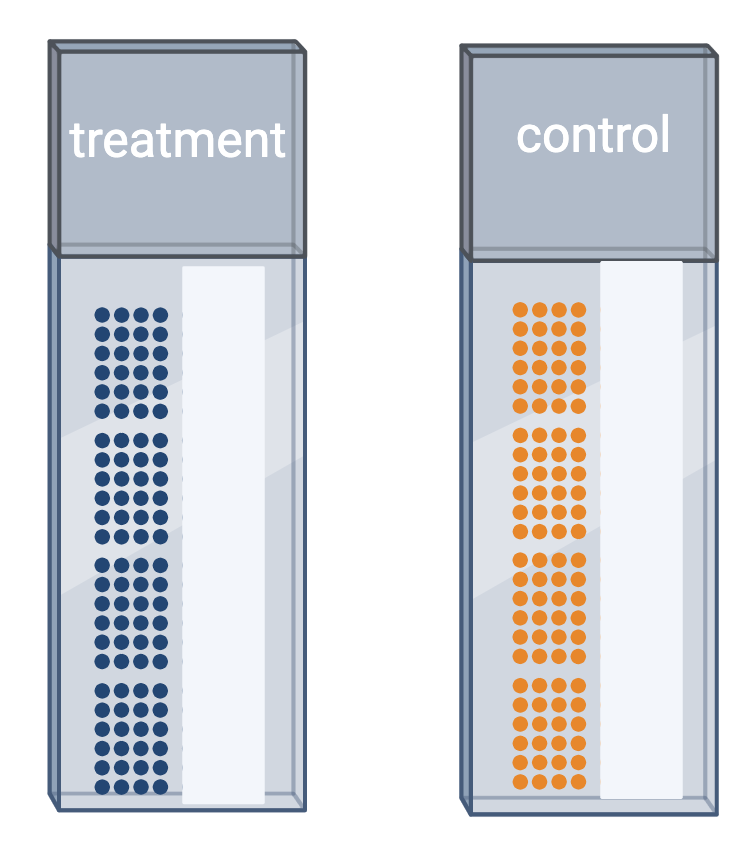
Challenge 6: Time points
Your study requires data collection at three time points: 5, 10, and 15 weeks. At the end of 5 weeks, you will run samples through the entire Visium workflow. You will repeat this for the 10- and 15-week samples when each of those time points is reached. What will happen when it is time for data analysis? What could you have done differently?
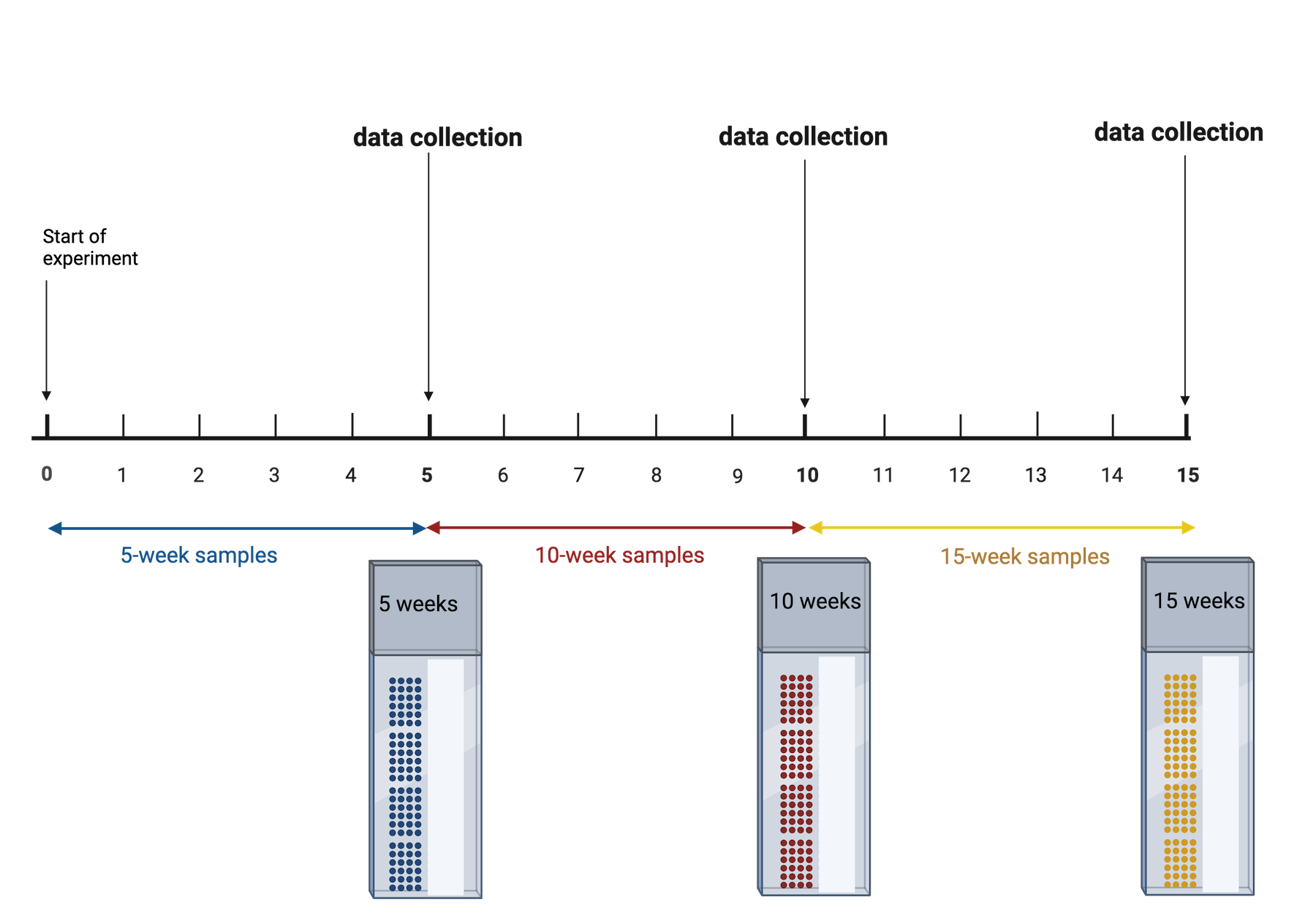
The issue is that time point is now confounded. A better approach would be to start the 15-week samples, then 5 weeks later start the 10-week samples, then 5 weeks later start the 5-week samples. This way you can run all of your samples at the same time. None of your samples will have spent a long time in the freezer, so you won’t need to worry about the variation that might cause. You won’t need to worry about the time point confounding the results.
Challenge 7: The efficient technician
Your technician colleague finds a way to simplify and expedite an
experiment. The experiment applies four different wheel-running
treatments to twenty different mice over the course of five days. Four
mice are treated individually each day for two hours each with a random
selection of the four treatments. Your clever colleague decides that a
simplified protocol would work just as well and save time. Run treatment
1 five times on day 1, treatment 2 five times on day 2, and so on. Some
overtime would be required each day but the experiment would be
completed in only four days, and then they can take Friday off! Does
this adjustment make sense to you?
Can you foresee any problems with the experimental results?
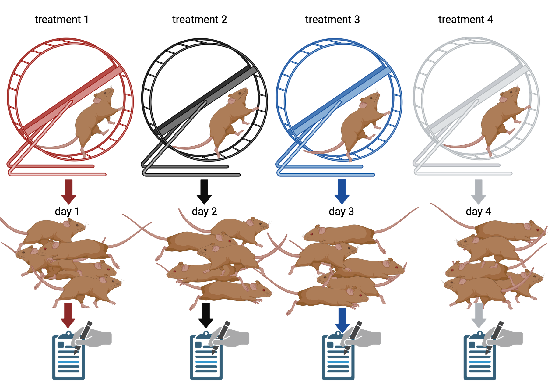
Since each treatment is run on only one day, the day effectively becomes the experimental unit (explain this). Each experimental unit (day) has five samples (mice), but only one replication of each treatment. There is no valid way to compare treatments as a result. There is no way to separate the treatment effect from the day-to-day differences in environment, equipment setup, personnel, and other extraneous variables.
Statistical power
Statistical power represents the probability of detecting a real treatment effect. Review the following figure to explore the relationships between effect size, sample size, and power. What is the relationship between effect size and sample size? Between sample size and power?
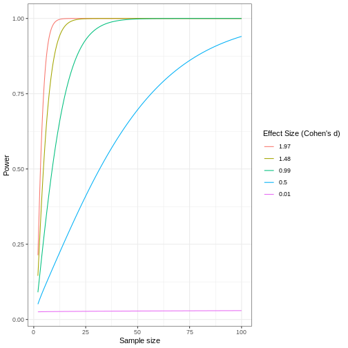
Adapted from How to Create Power Curves in ggplot by Levi Baguley
Notice that to detect a standardized effect size of 0.5 at 80% power, you would need a sample size of approximately 70. Larger effect sizes require much smaller sample sizes. Very small effects such as .01 never reach the 80% power threshold without enormous samples sizes in the hundreds of thousands.
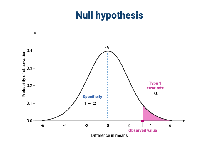
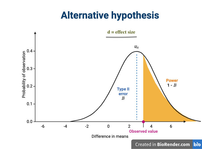
The effect size is shown in the figure above as the difference in means between the null and alternative hypotheses. Statistical power, also known as sensitivity, is the power to detect this effect.
To learn more about statistical power, effect sizes and sample size calculations, see Power and sample size by Krzywinski & Altman , Nature Methods 10, pages 1139–1140 (2013).
- Use
.mdfiles for episodes when you want static content - Use
.Rmdfiles for episodes when you need to generate output - Run
sandpaper::check_lesson()to identify any issues with your lesson - Run
sandpaper::build_lesson()to preview your lesson locally