Data Preprocessing
Last updated on 2025-10-07 | Edit this page
Estimated time: 95 minutes
Overview
Questions
- What data files should I expect from the Visium assay?
- Which data preprocessing steps are required to prepare the raw data files for further analysis?
- What software will we use for data preprocessing?
Objectives
- Explain how to use markdown with the new lesson template
- Demonstrate how to include pieces of code, figures, and nested challenge blocks
Introduction
The Space Ranger
software is a popular, though by no means only, set of pipelines for
preprocessing of Visium data. We focus on it here. It provides the
following output:
| File Name | Description |
|---|---|
| web_summary.html | Run summary metrics and plots in HTML format |
| cloupe.cloupe | Loupe Browser visualization and analysis file |
| spatial/ | Folder containing outputs that capture the spatiality of the data. |
| spatial/aligned_fiducials.jpg | Aligned fiducials QC image |
| spatial/aligned_tissue_image.jpg | Aligned CytAssist and Microscope QC image. Present only for CytAssist workflow |
| spatial/barcode_fluorescence_intensity.csv | CSV file containing the mean and standard deviation of fluorescence intensity for each spot and each channel. Present for the fluorescence image input specified by –darkimage |
| spatial/cytassist_image.tiff | Input CytAssist image in original resolution that can be used to re-run the pipeline. Present only for CytAssist workflow |
| spatial/detected_tissue_image.jpg | Detected tissue QC image. |
| spatial/scalefactors_json.json | Scale conversion factors for spot diameter and coordinates at various image resolutions |
| spatial/spatial_enrichment.csv | Feature spatial autocorrelation analysis using Moran’s I in CSV format |
| spatial/tissue_hires_image.png | Downsampled full resolution image. The image dimensions depend on the input image and slide version |
| spatial/tissue_lowres_image.png | Full resolution image downsampled to 600 pixels on the longest dimension |
| spatial/tissue_positions.csv | CSV containing spot barcode; if the spot was called under (1) or out (0) of tissue, the array position, image pixel position x, and image pixel position y for the full resolution image |
| analysis/ | Folder containing secondary analysis data including graph-based clustering and K-means clustering (K = 2-10); differential gene expression between clusters; PCA, t-SNE, and UMAP dimensionality reduction. |
| metrics_summary.csv | Run summary metrics in CSV format |
| probe_set.csv | Copy of the input probe set reference CSV file. Present for Visium FFPE and CytAssist workflow |
| possorted_genome_bam.bam | Indexed BAM file containing position-sorted reads aligned to the genome and transcriptome, annotated with barcode information |
| possorted_genome_bam.bam.bai | Index for possorted_genome_bam.bam. In cases where the reference transcriptome is generated from a genome with very long chromosomes (>512 Mbp), Space Ranger v2.0+ generates a possorted_genome_bam.bam.csi index file instead. |
| filtered_feature_bc_matrix/ | Contains only tissue-associated barcodes in MEX format. Each element of the matrix is the number of UMIs associated with a feature (row) and a barcode (column). This file can be input into third-party packages and allows users to wrangle the barcode-feature matrix (e.g. to filter outlier spots, run dimensionality reduction, normalize gene expression). |
| filtered_feature_bc_matrix.h5 | Same information as filtered_feature_bc_matrix/ but in HDF5 format. |
| raw_feature_bc_matrices/ | Contains all detected barcodes in MEX format. Each element of the matrix is the number of UMIs associated with a feature (row) and a barcode (column). |
| raw_feature_bc_matrix.h5 | Same information as raw_feature_bc_matrices/ in HDF5 format. |
| | raw_probe_bc_matrix.h5 |
| molecule_info.h5 | Contains per-molecule information for all molecules that contain a valid barcode, valid UMI, and were assigned with high confidence to a gene or protein barcode. This file is required for additional analysis spaceranger pipelines including aggr, targeted-compare and targeted-depth. |
Fortunately, you will not need to look at all of these files. We provide a brief description for you in case you are curious or need to look at one of the files for technical reasons.
The two files that you will use are
raw_feature_bc_matrix.h5 and
filtered_feature_bc_matrix.h5. These files have an
h5 suffix, which means that they are HDF5 files. HDF5 is
a compressed file format for storing complex high-dimensional data. HDF5
stands for Hierarchical Data Formats, version 5. There is an R
package designed to read and write HDF5 files called rhdf5.
This was one of the packages which you installed during the lesson
setup.
Briefly, HDF5 organizes data into directories within the
compressed file. There are three “files” within the HDF5
file:
| File Name | Description |
|---|---|
| features.csv | Contains the features (i.e. genes in this case) for each row in the data matrix. |
| barcodes.csv | Contains the probe barcodes for each spot on the tissue block. |
| matrix.mtx | Contains the counts for each gene in each spot. Features (e.g. genes) are in rows and barcodes (e.g. spots) are in columns. |
Set up Environment
Go to the File menu and select
Open Project. Open the spatialRNA project
which you created in the workshop setup.
First, we will load in some utility functions to make our lives a bit
easier. The source
function reads an R file and runs the code in it. In this case, this
will load several useful functions.
We will then load the libraries that we need for this lesson.
R
suppressPackageStartupMessages(library(tidyverse))
suppressPackageStartupMessages(library(hdf5r))
suppressPackageStartupMessages(library(Seurat))

source("https://raw.githubusercontent.com/smcclatchy/spatial-transcriptomics/main/code/spatial_utils.R")
Load Raw and Filtered Spatial Expression Data
In this course, we will use the Seurat R environment, which was
originally designed for analysis of single-cell RNA-seq data, but has
been extended for spatial transcriptomics data. The Seurat website
provides helpful vignettes
and a concise command cheat
sheet. SpatialExperiment
in R and scanpy
in python, amongst others, are also frequently used in analyzing spatial
transcriptomics data.
We will use the Load10X_Spatial
function from Seurat to read in the spatial transcriptomics data. These
are the data which you downloaded in the setup section.
First, we will read in the raw data for sample 151673.
R
raw_st <- Load10X_Spatial(data.dir      = "./data/151673",
                          filename      = "151673_raw_feature_bc_matrix.h5",
                          filter.matrix = FALSE)
If you did not see any error messages, then the data loaded in and
you should see an raw_st object in your
Environment tab on the right.
If the data does not load in correctly, verify that the students used the mode = “wb” argument in download.file() during the Setup. We have found that Windows users have to use this.
Let’s look at raw_st, which is a Seurat object.
R
raw_st
OUTPUT
An object of class Seurat
33538 features across 4992 samples within 1 assay
Active assay: Spatial (33538 features, 0 variable features)
 1 layer present: counts
 1 spatial field of view present: slice1
The output says that we have 33,538 features and 4,992 samples with one assay. Feature is a generic term for anything that we measured. In this case, we measured gene expression, so each feature is a gene. Each sample is one spot on the spatial slide. So this tissue sample has 33,538 genes assayed across 4,992 spots.
An experiment may have more than one assay. For example, you may run both RNA sequencing and chromatin accessibility in the same set of samples. In this case, we have one assay – RNA-seq. Each assay will, in turn, have one or more layers. Each layer stores a different form of the data. Initially, our Seurat object has a single counts layer, holding the raw, un-normalized RNA-seq counts for each spot. Subsequent downstream analyses can populate other layers, including normalized counts (conventionally stored in a data layer) or variance-stabilized counts (conventionally stored in a scale.data layer).
There is also a single image called slice1 attached to the Seurat object.
Next, we will load in the filtered data. Use the code above and look
in a file browser to identify the filtered file for sample
151673.
Challenge 1: Read in filtered HDF5 file for sample 151673.
Open a file browser and navigate to
Desktop/spatialRNA/data/151673. Can you find an HDF5 file
(with an .h5 suffix) that has the word “filtered” in
it?
If so, read that file in and assign it to a variable called
filter_st.
R
filter_st <- Load10X_Spatial(data.dir = "./data/151673",
                             filename = "151673_filtered_feature_bc_matrix.h5")
Once you have the filtered data loaded in, look at the object.
R
filter_st
OUTPUT
An object of class Seurat
33538 features across 3639 samples within 1 assay
Active assay: Spatial (33538 features, 0 variable features)
 1 layer present: counts
 1 spatial field of view present: slice1
The raw and filtered data both have the same number of genes (33,538). But the two objects have different numbers of spots. The raw data has 4,992 spots and the filtered data has 3,639 spots.
Look at the H&E slide below and notice the grey fiducial spots around the border. These are used by the spatial transcriptomics software to register the H&E image and the spatially-barcoded sequences.
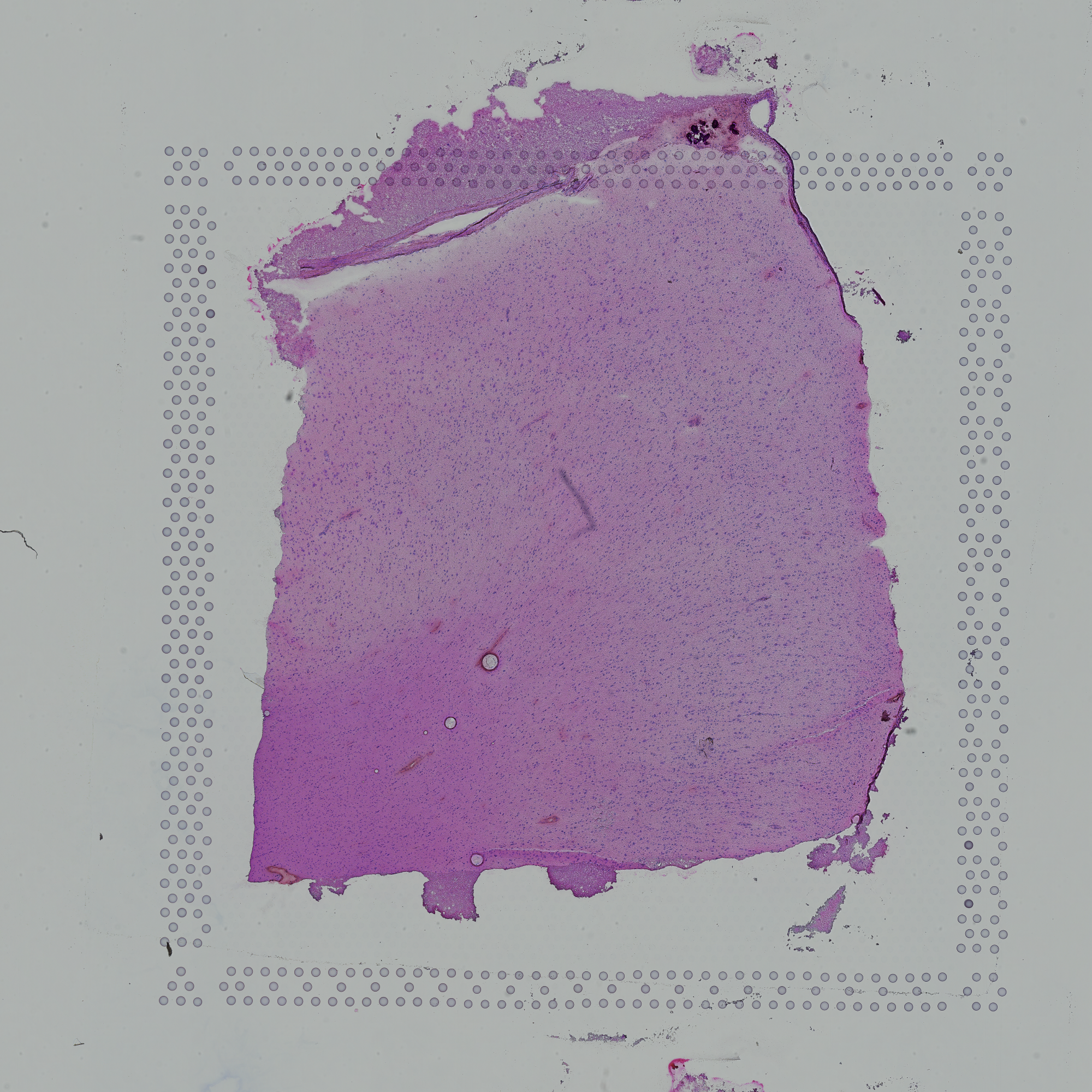
Challenge 2: How does the computer know how to orient the image?
Look carefully at the spots in the H&E image above. Are the spots symmetric? Is there anything different about the spots that might help a computer to assign up/down and left/right to the image?
Look at the spots in each corner. In the upper-left, you will see the following patterns:
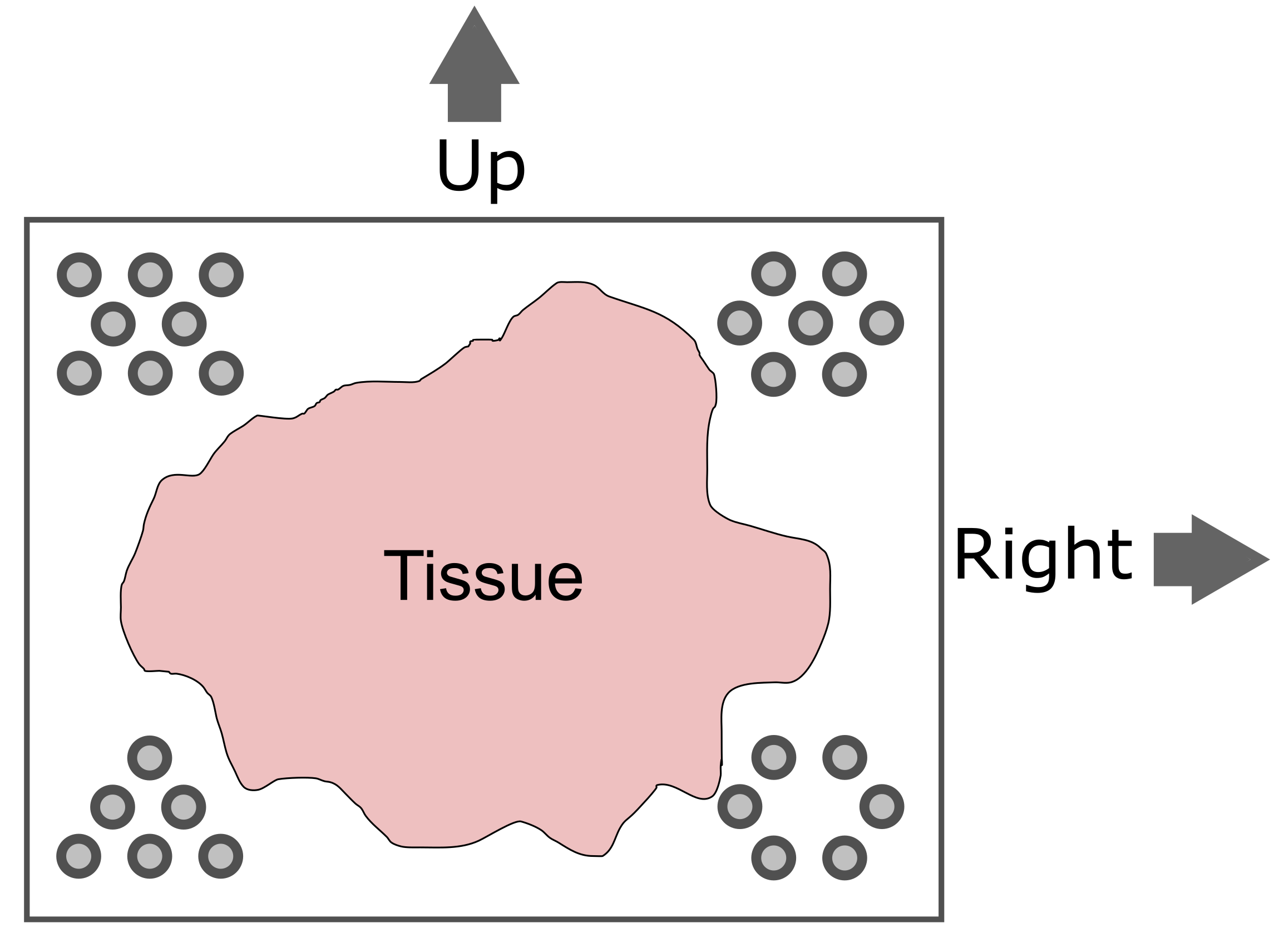
The patterns in each corner allow the spatial transcriptomics software to orient the slide.
Add Spot Metadata
The 10x Space Ranger pipeline automatically segments the tissue to
identify it within the background of the slide. This information is
encoded in the “tissue positions” file. Each row in the file corresponds
to a spot. The first column indicates whether the spot was (1) or was
not (0) identified as being within the tissue region by the segmentation
procedure. This file does not contain column names in earlier versions
of Space Ranger, but does starting with version SpaceRanger 2.0.
R
tissue_position <- read_csv("./data/151673/spatial/tissue_positions_list.csv",
                            col_names = FALSE, show_col_types = FALSE) %>%
                     column_to_rownames('X1')
colnames(tissue_position) <- c("in_tissue",
                               "array_row",
                               "array_col",
                               "pxl_row_in_fullres",
                               "pxl_col_in_fullres")
It is important to note that the order of the spots differs between
the Seurat object and the tissue position file. We need to reorder the
tissue positions to match the Seurat object. We can extract the spot
barcodes using the Cells
function. This is named for the earlier versions of Seurat, which
processed single cell transcriptomic data. In this case, we are getting
spot IDs, even though the function is called
Cells.
Next, we will add the tissue positions to the Seurat object’s metadata. Note that Seurat will align the spot barcodes in this process.
R
raw_st    <- AddMetaData(object = raw_st,    metadata = tissue_position)
filter_st <- AddMetaData(object = filter_st, metadata = tissue_position)
Next, we will plot the spot annotation, indicating spots that are in the tissue in blue and background spots in red.
R
SpatialPlot(raw_st, group.by = "in_tissue", alpha = 0.3)
WARNING
Warning: `aes_string()` was deprecated in ggplot2 3.0.0.
ℹ Please use tidy evaluation idioms with `aes()`.
ℹ See also `vignette("ggplot2-in-packages")` for more information.
ℹ The deprecated feature was likely used in the Seurat package.
  Please report the issue at <https://github.com/satijalab/seurat/issues>.
This warning is displayed once every 8 hours.
Call `lifecycle::last_lifecycle_warnings()` to see where this warning was
generated.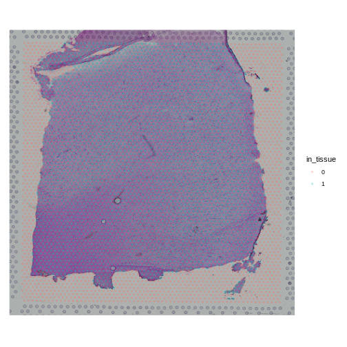
The 10x platform tags each molecule with a Unique Molecular
Identifier (UMI). This allows us to keep only one unique sequencing read
per molecule and to exclude those arising from PCR duplication. We
expect most of the UMI counts to be in the tissue spots. The Seurat
object metadata contains the UMI count in each spot in a column called
nCount_Spatial. Let’s plot the UMI counts in the tissue and
background spots.
R
raw_st@meta.data %>%
  ggplot(aes(as.logical(in_tissue), nCount_Spatial)) +
    geom_boxplot() +
    labs(title = 'UMI Counts in Tissue and Background',
         x     = 'In Tissue?',
         y     = 'Counts')
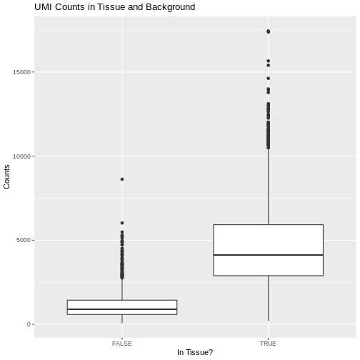
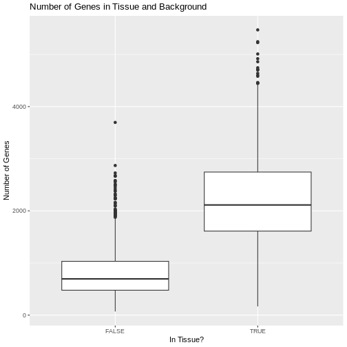
As expected, we see most of the counts in the tissue spots.
We can also plot the number of genes detected in each spot. Seurat
calls genes features, so we will plot the
nFeature_Spatial value. This is stored in the metadata of
the Seurat object.
R
raw_st@meta.data %>%
  ggplot(aes(as.logical(in_tissue), nFeature_Spatial)) +
    geom_boxplot() +
    labs(title = 'Number of Genes in Tissue and Background',
         x     = 'In Tissue?',
         y     = 'Number of Genes')
Challenge 3: Why might there be UMI counts outside of the tissue boundaries?
We expect UMI counts in the spots which overlap with the tissue section. What reasons can you think of that might lead UMI counts to occur in the background spots?
- When the tissue section is lysed, some transcripts may leak out of the cells and into the background region of the slide.
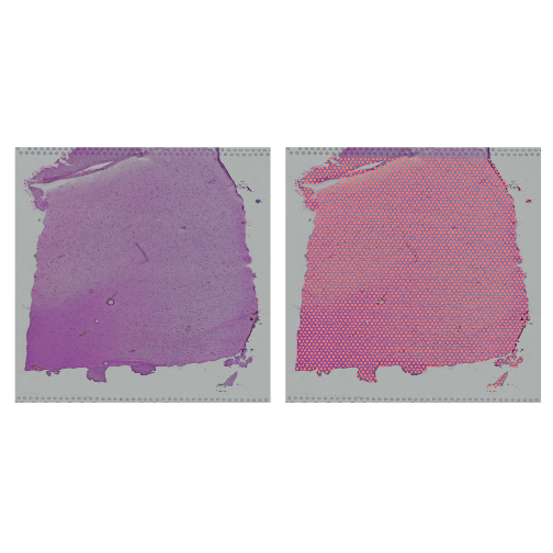
Up to this point, we have been working with the raw, unfiltered data to show you how the spots are filtered. However, in most workflows, you will work directly with the filtered file. From this point forward, we will work with the filtered data object.
Let’s plot the spots in the tissue in the filtered object to verify that it is only using spots in the tissue.
R
plot1 <- SpatialDimPlot(filter_st, alpha = c(0, 0)) +
           NoLegend()
plot2 <- SpatialDimPlot(filter_st) +
           NoLegend()
plot1 | plot2
Plot UMI and Gene Counts across Tissue
Next, we want to look at the distribution of UMI counts and numbers of genes in each spot across the tissue. This can be helpful in identifying technical issues with the sample processing.
It is useful to first think about what we expect. In the publication associated with this data, the authors show the structure that they expect in this tissue section of the human dorsolateral prefrontal cortex (DLPFC). In the figure below, they show a series of layers, from L1 to L6, arranged from the upper right to the lower left. In the lower left corner, they expect to see White Matter (WM). So we expect to see some series of layers arranged from the upper right to the lower left.
We will use Seurat’s SpatialFeaturePlot
function to look at these values. We can color the spots based on the
spot metadata stored in the Seurat object. You can find these column
names by looking at the meta.data slot of the Seurat
object.
R
head(filter_st@meta.data)
OUTPUT
                      orig.ident nCount_Spatial nFeature_Spatial in_tissue
AAACAAGTATCTCCCA-1 SeuratProject           8458             3586         1
AAACAATCTACTAGCA-1 SeuratProject           1667             1150         1
AAACACCAATAACTGC-1 SeuratProject           3769             1960         1
AAACAGAGCGACTCCT-1 SeuratProject           5433             2424         1
AAACAGCTTTCAGAAG-1 SeuratProject           4278             2264         1
AAACAGGGTCTATATT-1 SeuratProject           4004             2178         1
                   array_row array_col pxl_row_in_fullres pxl_col_in_fullres
AAACAAGTATCTCCCA-1        50       102               8468               9791
AAACAATCTACTAGCA-1         3        43               2807               5769
AAACACCAATAACTGC-1        59        19               9505               4068
AAACAGAGCGACTCCT-1        14        94               4151               9271
AAACAGCTTTCAGAAG-1        43         9               7583               3393
AAACAGGGTCTATATT-1        47        13               8064               3665
To plot the UMI counts, we will use the nCount_Spatial
column in the spot metadata.
R
plot1 <- SpatialDimPlot(filter_st, alpha = c(0, 0)) +
           NoLegend()
plot2 <- SpatialFeaturePlot(filter_st, features = "nCount_Spatial")
plot1 | plot2
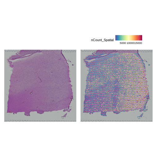
In this case, we see a band of higher counts running from upper left to lower right. There are also bands of lower counts above and below this band. The band in the upper right corner may be due to the fissure in the tissue. It is less clear why the expression is low in the lower-left corner.
We can also look at the number of genes detected in each spot using
nFeature_Spatial.
R
plot1 <- SpatialDimPlot(filter_st, alpha = c(0, 0)) +
           NoLegend()
plot2 <- SpatialFeaturePlot(filter_st, features = "nFeature_Spatial")
plot1 | plot2
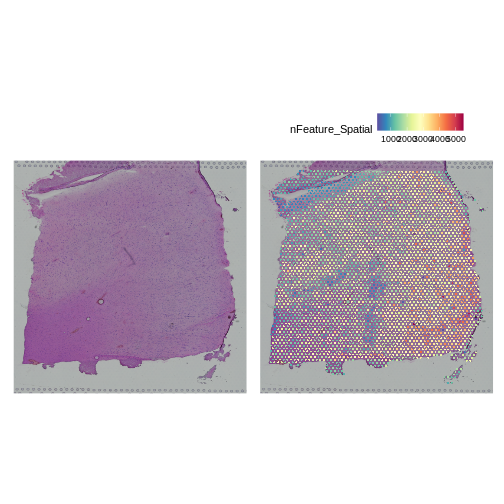
It is difficult to lay out a broad set of rules that will work for all types of tissues and samples. Some tissues may have homogeneous UMI counts across the section, while others may show variation in UMI counts due to tissue structure. For example, in cancer tissue sections, stromal cells tend to have lower counts than tumor cells and this should be evident in a UMI count plot. In the brain sample below, we might expect some variation in UMI counts in different layers of the brain.
Removing Genes with Low Expression
In order to build this lesson, we needed to reduce the size of the data. To do this, we are going to filter out genes that have no expression across the cells.
How many genes to we have before filtering?
R
paste(nrow(filter_st), "genes.")
OUTPUT
[1] "33538 genes."Next, we will get the raw counts, calculate the sum of each gene’s exprsssion across all spots, and filter the Seurat object to retain genes with summed counts greater than zero.
R
counts     <- LayerData(filter_st, 'counts')
gene_sums  <- rowSums(counts)
keep_genes <- which(gene_sums > 0)

filter_st  <- filter_st[keep_genes,]
WARNING
Warning: Not validating Centroids objects
Not validating Centroids objects
WARNING
Warning: Not validating FOV objects
Not validating FOV objects
Not validating FOV objects
Not validating FOV objects
Not validating FOV objects
Not validating FOV objects
WARNING
Warning: Not validating Seurat objectsHow many genes to we have after filtering?
R
paste(nrow(filter_st), "genes.")
OUTPUT
[1] "21842 genes."So we removed about 11,700 genes that had zero counts.
Conclusion
- The 10x Space Ranger pipeline provides you with an unfiltered and a filtered data file.
- The HDF5 file ends with an
h5extension and contains the barcodes, features (genes), and counts matrix. - Seurat is one of several popular environments for analyzing spatial transcriptomics data.
- It is important to know something about the structure of the tissue which you are analyzing.
- Plotting total counts and genes in each spot may help to identify quality control issues.