Deconvolution in Spatial Transcriptomics
Last updated on 2025-10-07 | Edit this page
Estimated time: 50 minutes
Overview
Questions
- How can we bring single-cell resolution to multi-cellular spatial transcriptomics spots?
- What are different algorithmic approaches for doing so?
Objectives
- Explain spot deconvolution.
- Perform deconvolution to quantify different cell types in spatial transcriptomics spots using a supervised approach that employs scRNA-seq data.
Deconvolution in Spatial Transcriptomics
Each spatial spot in an ST experiment generally contains multiple cells. For example, spots in the Visium assay are 55 microns in diameter, whereas a typical T cell has a diameter of ~10 microns. As such, the expression read out from the spot mixes together the expression of the individual cells encompassed by it. Deconvolution is the approach for unmixing this combined expression signal. Most often, deconvolution methods predict the fraction of each spot’s expression derived from each particular cell type. Supervised methods deconvolve spot expression using cell type expression profiles (e.g., from scRNA-seq) or marker genes. Therefore, we will need a prior knowledge or data for these methods. Unsupervised approaches instead infer the expression of the cell types without using priori information about cell types.
 Zhang
et al, Comput Struct Biotechnol J 21, 176–184 (2023)
CC
BY-NC-ND 4.0
Zhang
et al, Comput Struct Biotechnol J 21, 176–184 (2023)
CC
BY-NC-ND 4.0
Deconvolution with Robust Cell Type Decomposition (RCTD)
We will deconvolve spots by applying Robust Cell Type Decomposition
(RCTD; Cable, D.
M., et al., Nature Biotechnology, 2021), which is implemented in the
spacexr
package. The algorithm uses scRNA-seq data as a reference to deconvolve
the spatial transcriptomics data, estimating the proportions of
different cell types in each spatial spot. This method is considered
supervised method since we are using a prior knowledge about this
dataset. RCTD models the observed gene expression in each spatial spot
as a mixture of the gene expression profiles of different cell types,
where the estimated proportions are the coefficients of the expression
profiles in a linear model. Its procedure guarantees the
estimated proportions are non-negative, but note that they sum
to one. RCTD can operate in several modes: in doublet mode
it fits at most two cell types per spot, in full mode it
fits potentially all cell types in the reference per spot, and in
multi mode it again fits more than two cell types per spot
by extending the doublet approach. Here, we will use
full mode.
Loading scRNA-seq reference data
First, we load the scRNA-seq data that will serve as a reference for
deconvolution. Individual cells are assumed to be annotated according to
their type. RCTD will use these cell type-specific expression profiles
to deconvolve each spot’s expression. Please note the use of fread
from the data.table package. This provides an efficient means of loading
large data tables in csv and tsv format.
R
# # Load scRNA-seq data
sc.counts <- fread("data/scRNA-seq/sc_counts.tsv.gz") %>%
               column_to_rownames('V1') %>%
               as.matrix()

# Load cell type annotations
sc.metadata   <- read.delim("data/scRNA-seq/sc_cell_types.tsv")
sc.cell.types <- setNames(factor(sc.metadata$Value), sc.metadata$Name)

# Verify that the barcodes in counts and cell types match.
stopifnot(colnames(sc.counts) == names(sc.cell.types))
Next, we will create the reference object encapsulating this
scRNA-seq data. We will use the Reference
function, which will organize and store the scRNA-seq data for the next
steps.
R
sc_reference <- Reference(sc.counts, sc.cell.types)
Applying RCTD for spot deconvolution
Let’s write a wrapper function that performs RCTD deconvolution. This
will facilitate running RCTD on other samples within this dataset. It
calls SpatialRNA
to create an object representing the ST data, much as we did for the
scRNA-seq data with Reference above. It then links the ST
and scRNA-seq in an RCTD object created with create.RCTD
and finally performs deconvolution by calling run.RCTD.
R
# Write the wrapper function which takes the "reference" built above and calculates cell type propotions for current dataset, st.obj
run.rctd <- function(reference, st.obj) {

  # Get raw ST counts
  st.counts <- GetAssayData(st.obj, assay = "Spatial", layer = "counts")

  # Get the spot coordinates
  st.coords           <- st.obj[[]][, c("array_col", "array_row")]
  colnames(st.coords) <- c("x","y")

  # Create the RCTD 'puck', representing the ST data
  puck   <- SpatialRNA(st.coords, st.counts)

  myRCTD <- create.RCTD(puck, reference, max_cores = 1,
                        keep_reference = TRUE)

  # Run deconvolution -- note that we are using 'full' mode to devolve a spot
  # into (potentially) all available cell types.
  myRCTD <- suppressWarnings(run.RCTD(myRCTD, doublet_mode = 'full'))

  myRCTD
}
Running Deconvolution on Brain Samples
We apply the RCTD wrapper to our spatial transcriptomics data to deconvolve the spots and quantify the cell types. This may take ~10 minutes. If you prefer, you can load the precomputed results directly.
R
# Change this variable to TRUE to load precomputed results, or FALSE to
# compute the results here.
load.precomputed.results <- TRUE

rds.file <- paste0("data/rctd-sample-1.rds")

if(!load.precomputed.results || !file.exists(rds.file)) {

  result_1 <- run.rctd(sc_reference, sct_st)

  # The RCTD file is large. To save space, we will remove the reference
  # counts. This is necessary owing to constraints on sizes of files
  # uploaded to github during the automated build of this site. It will
  # not be required for your own analyses.
  # We use the remove.RCTD.reference.counts utility function defined in
  # code/spatial_utils.R.
  result_1 <- remove.RCTD.reference.counts(result_1)

  saveRDS(result_1, rds.file)

} else {

  result_1 <- readRDS(rds.file)

}
Interpreting Deconvolution Results
RCTD outputs the proportion of different cell types in each spatial
spot. These are held in the spatialRNA@counts slot. Let’s
see the proportions it predicts for this sample:
R
# Defining propotion of each cell type per spot.
props <- as.data.frame(result_1@results$weights)

# Print the first few lines of the deconvolution results
# Each row is a spot and each column is propotion of each cell type in that spot
head(props)
OUTPUT
                      AST-FB         L2-3           L4         L5-6
AAACAAGTATCTCCCA-1 0.2906892 1.989539e-01 3.568361e-01 9.495123e-04
AAACAATCTACTAGCA-1 0.3665241 4.652610e-04 4.652610e-04 4.601510e-01
AAACACCAATAACTGC-1 0.1069532 5.473749e-05 5.473749e-05 5.473749e-05
AAACAGAGCGACTCCT-1 0.3845201 4.758347e-01 3.256827e-04 3.256827e-04
AAACAGCTTTCAGAAG-1 0.2411203 3.694851e-01 1.995963e-01 6.646586e-04
AAACAGGGTCTATATT-1 0.2096408 3.256827e-04 3.624793e-04 5.117059e-01
                   Oligodendrocytes
AAACAAGTATCTCCCA-1       0.04291383
AAACAATCTACTAGCA-1       0.12784650
AAACACCAATAACTGC-1       1.25940541
AAACAGAGCGACTCCT-1       0.06181266
AAACAGCTTTCAGAAG-1       0.23374357
AAACAGGGTCTATATT-1       0.46602478
Notice that the proportions don’t sum exactly to one:
R
# Print sum of cell type propotions in each spot
head(rowSums(props))
OUTPUT
AAACAAGTATCTCCCA-1 AAACAATCTACTAGCA-1 AAACACCAATAACTGC-1 AAACAGAGCGACTCCT-1
         0.8903426          0.9554521          1.3665228          0.9228188
AAACAGCTTTCAGAAG-1 AAACAGGGTCTATATT-1
         1.0446099          1.1880596
Let’s classify each spot according to the layer type with highest proportion:
R
# Classifying each spot based on the maximum propotion of a cell type in that spot.
props$classification <- colnames(props)[apply(props, 1, which.max)]
Let’s add the deconvolution results to our Seurat object, so that they can be visualized and analyzed alongside other data organized there.
R
# Adding cell type propotions to seurat object.
sct_st <- AddMetaData(object = sct_st, metadata =  props)
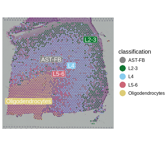
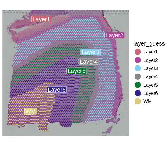
We can now visualize the predicted layer classifications and compare them alongside the authors’ annotations that we saw previously.
R
# Plot classification of each spot based on RCTD results.
SpatialDimPlotColorSafe(sct_st[, !is.na(sct_st[[]]$classification)],
                        "classification")
R
# Plot classification of each spot based on annotation of a biologist.
SpatialDimPlotColorSafe(sct_st[, !is.na(sct_st[[]]$layer_guess)],
                        "layer_guess")
To be more quantitative, we can compute a confusion matrix comparing the layers predicted by RCTD with those annotated by the authors.
R
# Compare predictions from RCTD with annotation done by biologist.
df            <- as.data.frame(table(sct_st[[]]$layer_guess,
                                     sct_st[[]]$classification))
colnames(df)  <- c("Annotation", "Prediction", "Freq")
df$Annotation <- factor(df$Annotation)
df$Prediction <- factor(df$Prediction)

ggplot(data = df, aes(x = Annotation, y = Prediction, fill = Freq)) +
  geom_tile() +
  theme(text = element_text(size = 20),
        axis.text.x = element_text(angle = 45, vjust = 1, hjust=1))
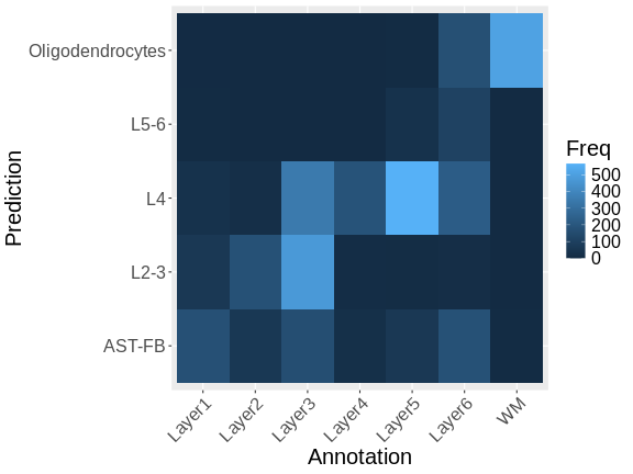
Note that there is a fairly strong correlation between the predicted and observed layers, particularly for the pairs Oligodendrocytes and WM (White Matter), L4 and Layer 4, and L2-3 and Layer 3.
Summary
Deconvolution quantifies the cell type composition of each spot. Doing so enables downstream analyses, such as the proportion of various cell types across a sample, heterogeneity of cell types across the sample, or co-localization analyses of cell types within the sample. Supervised (i.e., reference-based) and unsupervised approaches have been developed.
Here, we applied deconvolution supervised by scRNA-seq annotations, as implemented in RCTD, to a brain sample. The highly structured organization of the brain allows clear visual confirmation of deconvolution results. Other tissues may have less structure and more intermingling of cell types. For example, a typical use of deconvolution in a cancer setting is to explore co-localization of tumor and immune cells.
- Deconvolution enhances spatial transcriptomics by quantifying the different cell types within spatial spots.
- Integrating scRNA-seq data with spatial transcriptomics data facilitates accurate deconvolution.
- RCTD is a supervised deconvolution method that quantifies the proportion of different cell types in spatial transcriptomics data.