Performing a Genome Scan with Binary Traits

Estimated time: 50 minutes

Overview

Questions

• How do I perform a genome scan for binary traits?

Objectives

• Convert phenotypes to binary values.
• Use logistic regression for genome scans with binary traits.
• Plot and compare genome scans for binary traits.

Binary Phenotypes

---

The genome scans in the previous episode were performed assuming that the residual variation followed a normal distribution. This will often provide reasonable results even if the residuals are not normal, but an important special case is that of a binary trait, with values 0 and 1, which is best treated differently. The scan1 function can perform a genome scan with binary traits by logistic regression, using the argument model="binary". (The default value for the model argument is "normal"). At present, we cannot account for kinship relationships among individuals in this analysis.

Let’s look at the phenotypes in the cross again.

R

head(cross$pheno)

OUTPUT

          log10_insulin_10wk agouti_tan tufted
Mouse3051              1.399          1      0
Mouse3551              0.369          1      1
Mouse3430              0.860          0      1
Mouse3476              0.800          1      0
Mouse3414              1.370          0      0
Mouse3145              1.783          1      0

There are two binary traits called agouti_tan and tufted which are related to coat color and shape.

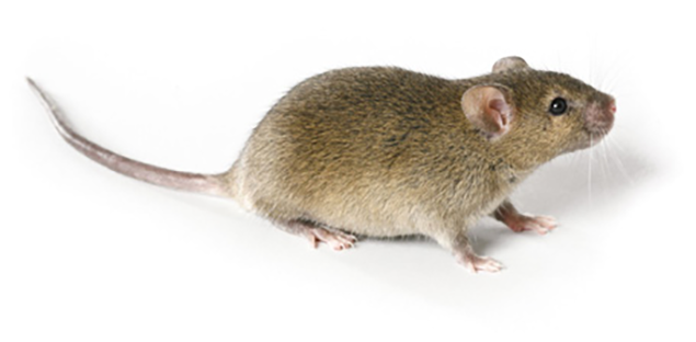
The agouti_tan phenotype is 1 if a mouse has an agouti or tan coat and 0 if a mouse has a black coat. The founder strains have different coat colors. C57BL/6J has a black coat.

C57BL/6J

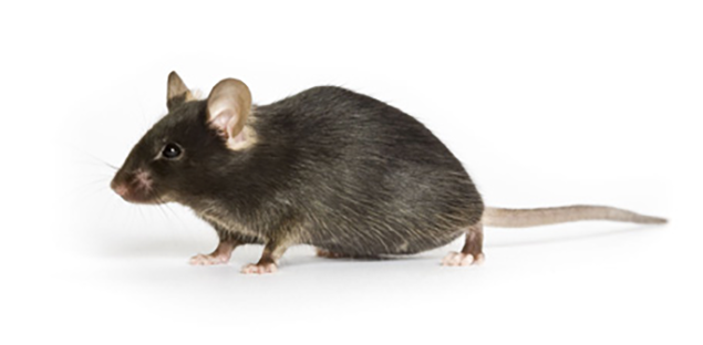
BTBR appears to have a black coat, but this coat color is actually called “black and tan” because their bellies are tan.

BTBR

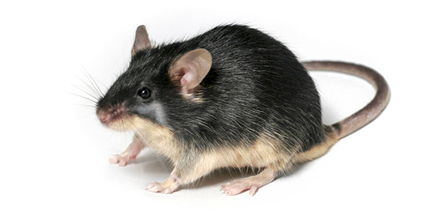
Agouti mice appear to be tan or brown, but their hair is a mix of brown and black coloring. As an example, C3H/HeJ mice have agouti coats.

C3H/HeJ

There is more information about mouse coat colors in the JAX Coat Color guide.

The tufted phenotype has to do with progressive hair loss in a “tufted” pattern. Mice with a value of 1 have the tufted phenotype and mice with a value of 0 do not.

Tufted hair loss pattern

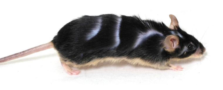
Photo Credit: Ellis et al., J Hered, 2013

Performing a Binary Genome Scan

---

We perform a binary genome scan in a manner similar to mapping continuous traits by using scan1. When we mapped insulin, there was a hidden argument called model which told qtl2 which mapping model to use. There are two options: normal, the default, and binary. The normal argument tells qtl2 to use a normal (least squares) linear model. To map a binary trait, we will include the model = "binary" argument to indicate that the phenotype is a binary trait with values 0 and 1.

R

lod_agouti <- scan1(genoprobs = probs, 
                    pheno     = cross$pheno[,'agouti_tan', drop = FALSE], 
                    addcovar  = addcovar, 
                    model     = "binary")

Let’s plot the result and see if there is a peak.

R

plot_scan1(x    = lod_agouti, 
           map  = cross$pmap, 
           main = 'Agouti')

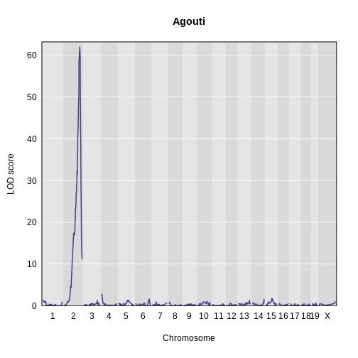
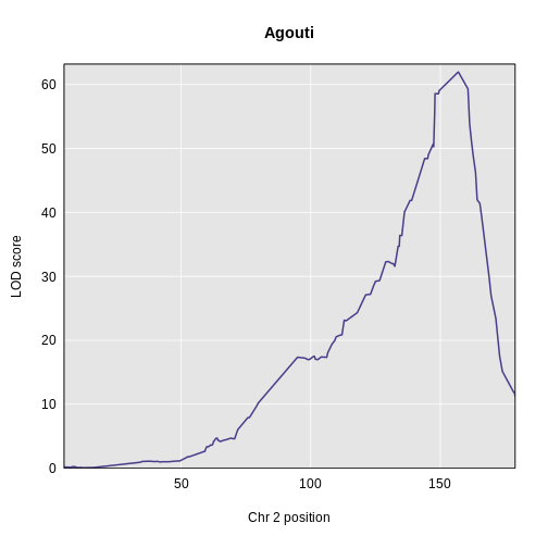
Yes! There is a big peak on chromosome 2. Let’s zoom in on chromosome 2.

R

plot_scan1(x    = lod_agouti, 
           map  = cross$pmap, 
           chr  = "2",
           main = "Agouti")

We can use find_peaks to find the position of the highest LOD score.

R

find_peaks(scan1_output = lod_agouti, 
           map          = cross$pmap)

OUTPUT

  lodindex  lodcolumn chr pos  lod
1        1 agouti_tan   2 157 61.9

This turns out to be a well-known coat color locus for agouti coat color which contains the nonagouti gene. Mice carrying two black alleles will have a black coat, and mice carrying one or no black alleles will have agouti coats.

Challenge 1: How many mice have black coats?

Look at the frequency of the black (0) and agouti (1) phenotypes. What proportion of the mice are black? Can you use what you learned about how the nonagouti locus works and the cross design to explain the frequency of black mice?

Show me the solution

First, get the number of black and agouti mice.

R

tbl <- table(cross$pheno[,"agouti_tan"])
tbl

OUTPUT

  0   1
125 356 

Then use the number of mice to calculate the proportion with each coat color.

R

tbl / sum(tbl)

OUTPUT

   0    1
0.26 0.74 

We can see that the black (0) mice occur about 25 % of the time. If the B allele causes mice to have black coats when it is recessive, and if R is the agouti allele, then, when breeding two heterozygous (BR) mice together, we expect the following genotypes in the progeny:

/	B	R
B	BB	BR
R	BR	RR

Hence, we expect mean allele frequencies and coat colors as follows:

Allele	Frequency	Coat Color
BB	0.25	black
BR	0.50	agouti
RR	0.25	agouti

From this, we can see that about 25% of the mice should have black coats.

Challenge 2: Map the “tufted” phenotype.

Map the tufted phenotype an determine if there are any tall peaks for this trait.

Show me the solution

First, map the trait.

R

lod_tufted <- scan1(genoprobs = probs, 
                    pheno     = cross$pheno[,"tufted", drop = FALSE], 
                    addcovar  = addcovar, 
                    model     = "binary")

Then, plot the LOD score.

R

plot_scan1(x    = lod_tufted, 
           map  = cross$pmap, 
           main = "Tufted")

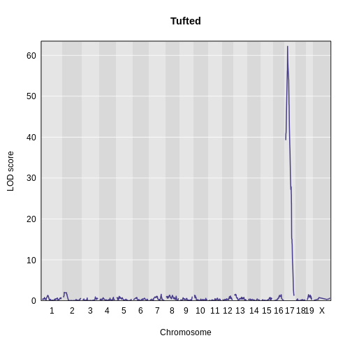
Finally, use find_peaks to get the peak LOD location.

R

find_peaks(scan1_output = lod_tufted, 
           map          = cross$pmap)

OUTPUT

  lodindex lodcolumn chr  pos  lod
1        1    tufted  17 27.3 62.2

There is a large peak on chromosome 17. This is a known locus associated with the Itpr3 gene near 27.3 Mb on chromosome 17.

Key Points

• A genome scan for binary traits (0 and 1) requires special handling; scans for non-binary traits assume normal variation of the residuals.
• A genome scan for binary traits is performed using logistic regression.