Mapping Many Gene Expression Traits
Last updated on 2025-09-30 | Edit this page
Estimated time: 50 minutes
Overview
Questions
- How do I map all of the genes in my data set?
- What resources do I need to map all of the genes in my data set?
Objectives
- To map several genes at the same time
Mapping All Genes
Most people have laptops with enough memory and computing power to map hundreds of genes. However, we have over 20,000 genes in our data set. This would either take a very long time or would use up all of the memory on most peoples’ laptops.
To map all of the genes, you will need to use a computing cluster, such as sumner2 at JAX. Since mapping all of the genes took 12 hours, you will not perform this operation in this workshop. Instead, we will show you how to set up a computing job to run this analysis.
sumner2 uses slurm to schedule
computing jobs. slurm is software that runs on the cluster
and manages how computing jobs are run. Users submit job requests and
slurm checks whether the requested memory, number of
processors, and time are available and then decides when to run the job.
It also balances the needs of different users so that everyone can get
their computing jobs done.
sumner2 also uses software containers to run software. JAX
uses Singularity
containers. These contain software without the need to install it on the
cluster. The Computational Sciences group makes a large number of
containers available on sumner2 and we will use their
qtl2 container.
If you are unfamiliar with the JAX computing cluster, Research IT has
excellent
documentation that explains how the cluster works, how to submit
jobs using slurm, and how to use Singularity
containers.
bash Script
To run a batch job on the cluster, we will create a bash script which
will request resources from slurm and will call an R
script, which will perform the mapping. The script that we used is shown
below.
#!/bin/bash
#SBATCH --qos batch
#SBATCH --partition compute
#SBATCH --nodes 1
#SBATCH --ntasks 1
#SBATCH --cpus-per-task 22
#SBATCH --mem 200G
#SBATCH --time 1-0:00

CONTAINER=/projects/omics_share/meta/containers/quay.io-jaxcompsci-r-qtl2-deseq-biomart-tidy-v4.img

module load singularity

singularity exec ${CONTAINER} Rscript eqtl.R
For each data set, you will need to determine the number of cores to
use. qtl2 can perform the QTL mapping in parallel on one
node, so you will typically request only one node. In this case, we
requested 22 cores on one node. sumner2 has nodes with up to 70
cores, but there is a point of diminishing returns when parallelizing
too much. We performed a short test run and found that we used about
100GB of memory, so we requested twice that amount in case there were
memory surges during computation. And we requested one day (24 hours) of
compute time.
Overall, the job took 12 hours and used 100GB of memory.
Note that there are many ways to set up a computing job, including
starting many separate mapping jobs and combining the results. We have
chosen to show you one simple way in this course. If you have
slurm expertise, you can try other methods of breaking up
the work.
Next, we call the R script using singularity exec to
execute the command which follows the container name. We call
Rscript to run the eQTL mapping script, which we placed in
the same directory as the bash script.
The inputs to the script are the genoprobs, expression data, covariates, kinship matrix, and the marker map. You should have all of these pre-computed and saved on the cluster in the same directory.
R Script
################################################################################
# Script to map all of the Attic DO 500 pancreatic islet RNASeq data.
#
# Daniel Gatti
# dan.gatti@jax.org
# 2024-11-01
################################################################################

##### LIBRARIES #####

library(qtl2)

##### VARIABLES #####

# Base directory for project.
base_dir = '/projects/compsci/eqtl_course'

# Number of cores. MUST MATCH SLURM REQUEST.
n_cores = 20

# Read in pre-built data files.

probs = readRDS(file.path(base_dir, 'attie_DO500_genoprobs_v5.rds'))
K     = readRDS(file.path(base_dir, 'attie_do_kinship.rds'))
covar = readRDS(file.path(base_dir, 'attie_do_covar.rds'))
expr  = readRDS(file.path(base_dir, 'attie_do_expr_rz.rds'))
map   = readRDS(file.path(base_dir, 'attie_do_map.rds'))

##### MAIN #####

# Convert covariates to factors.
covar$sex    = factor(covar$sex)
covar$DOwave = factor(covar$DOwave)

# Create a matrix of additive covariates.
addcovar     = model.matrix(~sex + DOwave, data = covar)[,-1]

# Map all genes.
lod = scan1(genoprobs = probs,
            pheno     = expr,
            kinship   = K,
            addcovar  = addcovar,
            cores     = n_cores)

# Save the LOD scores for all genes.
saveRDS(lod, file = file.path(base_dir, 'attie_do_eqtl_lod.rds'))

# Get the peaks with LOD >= 6.
peaks = find_peaks(scan1_output = lod,
                   map          = map,
                   threshold    = 6,
                   prob         = 0.95)

# Save the harvested LOD peaks.
saveRDS(peaks, file = file.path(base_dir, 'attie_do_eqtl_peaks.rds'))
The output of this script is two files.
-
attie_do_eqtl_lod.rds: This is numeric matrix containing LOD scores for all genes at all markers. We save it as a compressed R data file (*.rds). In this case, the file is 11 GB. -
attie_do_eqtl_peaks.rds: This is a data.frame containing the peaks with LOD over 6. We save it as a compressed R data file (*.rds). In this case, the file is 674 KB. You should have downloaded this file into yourdatadirectory.
Finding QTL Peaks
Let’s load in the QTL peaks that we pre-computed.
R
peaks <- readRDS(file = "data/attie_do_eqtl_peaks.rds")
peaks is a data frame which contains all of the peaks in
the same format as we saw in the previous lesson. Let’s remind ourselves
what the peaks table looks like.
R
head(peaks)
OUTPUT
  lodindex          lodcolumn chr       pos       lod      ci_lo     ci_hi
1        2 ENSMUSG00000000028   6  71.73759  7.402989  65.005336  77.42623
2        2 ENSMUSG00000000028  11  40.55159  6.028608   3.031502 119.01535
3        2 ENSMUSG00000000028  16  18.54468  7.875773  15.918386  20.81798
4        3 ENSMUSG00000000037   5  99.00918  6.837536  93.289032  99.67072
5        3 ENSMUSG00000000037  12  77.55794  6.153038  77.002567 110.22383
6        3 ENSMUSG00000000037   X 161.30209 26.698858 160.417579 161.80999
Each row contains information for one peak, including the gene ID, chromosome, peak position, LOD, and support interval.
Notice that both genes ENSMUSG00000000028 and
ENSMUSG00000000037 have more than one peak.
Challenge 1: How many genes have QTL peaks?
Look at how many genes we have and how many rows there are in peaks. Is this the same number? If not, can you explain why the numbers are different.
Get the number of genes from expr_rz.
R
ncol(expr_rz)
OUTPUT
[1] 21771Get the number of QTL peaks in peaks.
R
nrow(peaks)
OUTPUT
[1] 42941There are more peaks than there are genes.
There are several different possibilities when mapping a gene.
- A gene may have no QTL peaks over a LOD of 6, and so it will not appear in the list of peaks.
- A gene may have more than one QTL peak with a LOD greater than 6, and so will appear many times in the list of peaks.
Let’s count the number of peaks that each gene has.
R
dplyr::count(peaks, lodcolumn) |>
  dplyr::count(n)
OUTPUT
    n   nn
1   1 9201
2   2 6755
3   3 3789
4   4 1425
5   5  483
6   6   87
7   7   25
8   8    4
9   9    1
10 10    1
From the table above, we can see that most genes have one or two peaks. However, some genes have 9 peaks with LOD > 6!
When we built this table, we selected all of the peaks with LOD > 6. This is well below the alpha = 0.05 significance threshold. Let’s get that threshold and filter the list of peaks.
R
ethr <- summary(object = eperm,
                alpha  = 0.05)
ethr
OUTPUT
LOD thresholds (1000 permutations)
     ENSMUSG00000020679
0.05               7.47
Now filter the peaks to retain peaks with LOD greater than or equal to 7.4745761.
R
peaks_filt <- filter(peaks, lod >= ethr[1,1])
Challenge 2: How many peaks are there after filtering?
Get the number of QTL peaks that we have after filtering.
R
nrow(peaks_filt)
OUTPUT
[1] 17164There are now fewer peaks.
Challenge 3: How many peaks does each gene have?
Use the code above to count the number of QTL peaks that each gene has.
R
dplyr::count(peaks_filt, lodcolumn) |>
  dplyr::count(n)
OUTPUT
  n    nn
1 1 12707
2 2  1959
3 3   151
4 4    19
5 5     2
Now most genes have only one peak and only two genes have five peaks.
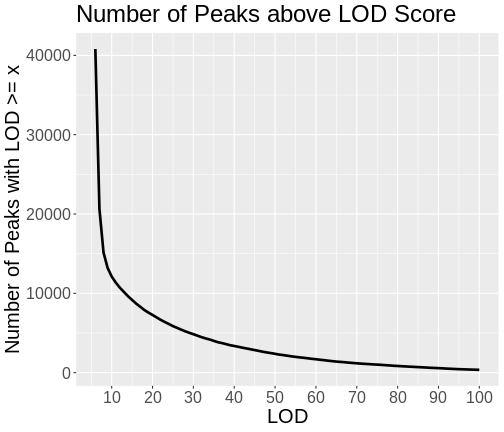
Let’s look at the number of genes with LOD scores above a certain value. We do this by counting the number of peaks with LOD > 6, then > 7, etc.
Do not try to type the next block. We will look at it on the workshop website.
R
lod_brks <- 1:100
results  <- data.frame(lod_brks, n = 0)

for(i in lod_brks) {

  results$n[i] <- sum(peaks$lod >= i)

} # for(i)

results |>
  filter(lod_brks >= 6) |>
  ggplot(aes(lod_brks, n)) +
    geom_line(linewidth = 1.25) +
    scale_x_continuous(breaks = 0:10 * 10) +
    labs(title = "Number of Peaks above LOD Score",
         x     = "LOD",
         y     = "Number of Peaks with LOD >= x") +
    theme(text = element_text(size = 20))

R
rm(lod_brks, results)
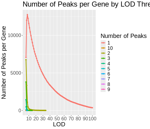
As you can see from the plot above, most peaks have LODs less than 10. However, about 12,000 peaks have LODs over 10. As we increase the LOD score, we see that fewer genes have high LODs. Let’s look at how many peaks each gene has as we increase the LOD threshold.
Do not try to type the next block. We will look at it on the workshop website.
R
lod_brks <- 0:100
result   <- data.frame(lod_brks = -1, n = 0, nn = 0)

for(i in lod_brks) {
  smry <- peaks |>
            filter(lod > i) |>
            dplyr::count(lodcolumn) |>
            dplyr::count(n) |>
            mutate(lod_brks = i)

  result <- bind_rows(result, smry)
} # for(i)

result |>
  filter(lod_brks >= 6) |>
  mutate(n = as.character(n)) |>
  ggplot(aes(lod_brks, nn, color = n)) +
    geom_line(aes(group = n), size = 1.25) +
    geom_point() +
    scale_x_continuous(breaks = 0:10 * 10) +
    labs(title = "Number of Peaks per Gene by LOD Threshold",
         x     = "LOD",
         y     = "Number of Peaks per Gene",
         color = "Number of Peaks") +
    theme(text = element_text(size = 20))

R
rm(lod_brks, result)
From this plot, we can see that higher LOD scores occur only once per gene. This makes sense since a high LOD score implies that the peak explains a large proportion of the gene’s variance.
Summary
In this episode, you learned how to run an eQTL analysis on a computing cluster and started to look at the resulting peaks. When we filter the peaks by higher LOD scores, we tend to get fewer peaks per gene.
- Mapping all genes in a study requires a computing cluster.
- Genes may have more than one QTL peak.
- High LOD scores often occur only once per gene.
