Mediation Analysis
Last updated on 2025-10-07 | Edit this page
Estimated time: 80 minutes
Overview
Questions
- What is mediation analysis?
- How do I explore causal relations with mediation analysis?
Objectives
- Describe mediation analysis as applied in genetics and genomics.
R
library(knitr)
library(tidyverse)
library(qtl2)

pheno      <- readRDS(file = 'data/attie_do_pheno.rds')
pheno_dict <- readRDS(file = 'data/attie_do_pheno_dict.rds')
covar      <- readRDS(file = 'data/attie_do_covar.rds')
covar$DOwave <- factor(covar$DOwave)
addcovar   <- model.matrix(~sex + DOwave, data = covar)[,-1]
annot      <- readRDS(file = 'data/attie_do_expr_annot.rds')
expr_rz    <- readRDS(file = 'data/attie_do_expr_rz.rds')
map        <- readRDS(file = 'data/attie_do_map.rds')
probs      <- readRDS(file = url('https://thejacksonlaboratory.box.com/shared/static/4hy4hbjyrxjbrzh570i4g02r62bx3lgk.rds'))
K          <- readRDS(file = 'data/attie_do_kinship.rds')
ins_tauc   <- pheno[, 'Ins_tAUC', drop = FALSE]
ins_tauc$Ins_tAUC_log <- log(ins_tauc$Ins_tAUC)
ins_lod    <- readRDS(file = 'data/ins_tauc_lod.rds')
eperm      <- readRDS(file = 'data/ENSMUSG00000020679_perm_1000.rds')
hotspots   <- readRDS(file = 'data/eqtl_hotspots.rds')
pc1_2      <- readRDS(file = 'data/eqtl_hotspot_chr2_pc1.rds')
pc1_lod    <- readRDS(file = 'data/eqtl_hotspot_chr2_pc1_lod.rds')
Introduction
GWAS studies show that most disease-associated variants are found in non-coding regions. This fact leads to the idea that regulation of gene expression is an important mechanism enabling genetic variants to affect complex traits. Mediation analysis can identify a causal chain from genetic variants to molecular and clinical phenotypes. The graphic below shows complete mediation, in which a predictor variable does not directly impact the response variable. Rather, it directly influences the mediator (path a). The mediator has a direct impact on the response variable (path b). We would see (path c) the relationship between predictor and response, not knowing that a mediator intervenes in this relationship.
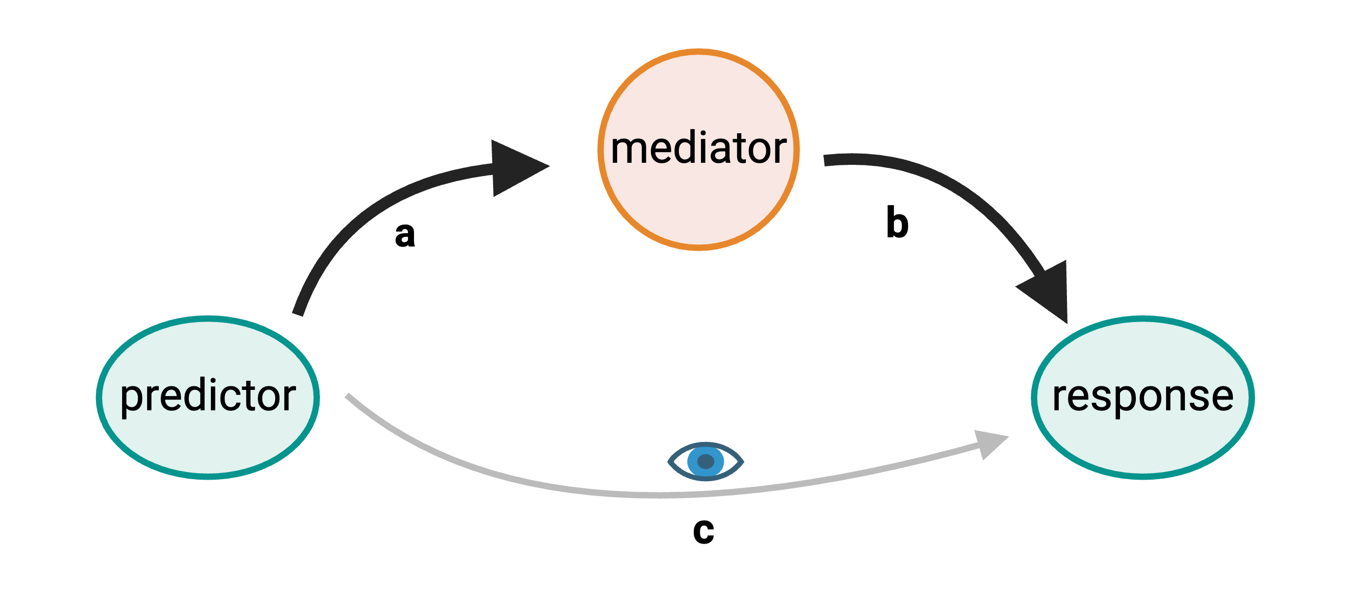
Mediation analysis is widely used in the social sciences including psychology. In biomedicine, mediation analysis has been employed to investigate how gene expression mediates the effects of genetic variants on complex phenotypes and disease.
For example, a genetic variant (non-coding SNP) indirectly regulates expression of gene 2 through a mediator, gene 1. The SNP regulates expression of gene 1 locally, and expression of gene 1 influences expression of gene 2 distally.
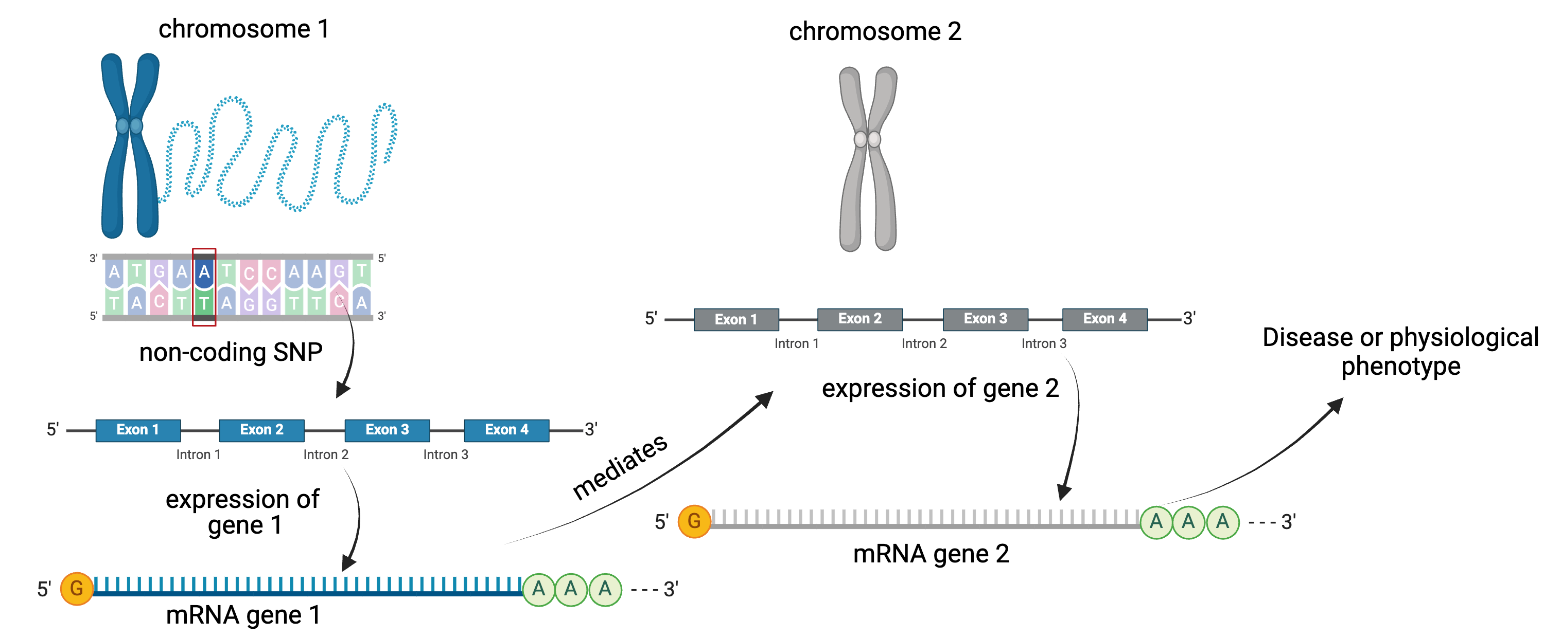
Instead of the expression of one gene impacting another, expression of gene 1 in the graphic above could impact a physiological phenotype like blood glucose. Expression of gene 1 would mediate the relationship between the non-coding SNP and the glucose phenotype.
Gene Akr1e1 is located on chromosome 13 in mouse.
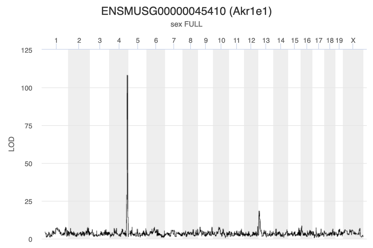
Challenge 1: Interpreting Akr1e1 eQTL plot.
How would you interpret the Akr1e1 LOD plot above? On which chromosome(s) would you expect to find the driver gene(s)? The SNP(s)?
Ark1e1 expression is regulated by some variants on chromosome 13 and other variants on chromosome 4. The largest driver gene occurs on chromosome 4 because the LOD peak is higher there, indicating that the genotype on chromosome 4 explains more of the variance than the one on chromosome 13.
Myo15b is located on chromosome 11.
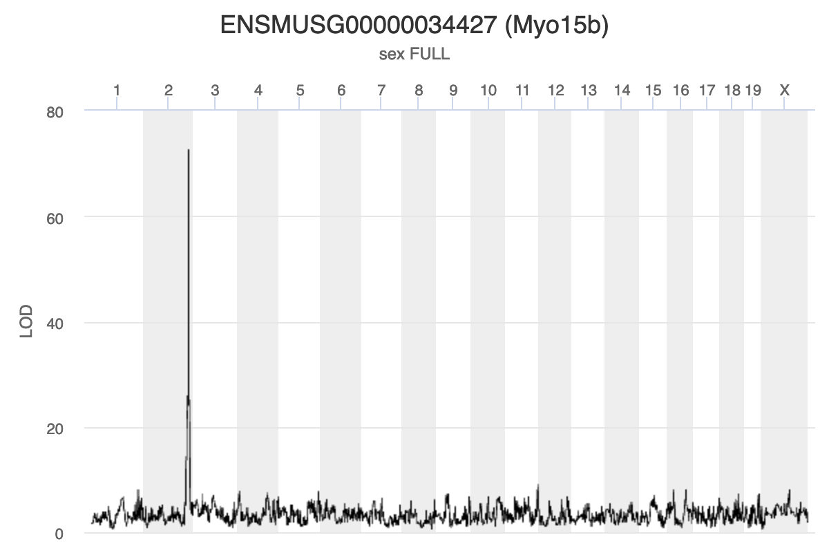
Challenge 2: Interpreting Myo15b eQTL plot.
How would you interpret the Myo15b LOD plot above? On which chromosome(s) would you expect to find the driver gene(s)? The SNP(s)?
Myo15b is regulated by variants on chromosome 2 because the largest LOD peak is located there.
Using Gene Expression as a Covariate
When we are searching for a gene whose expression influences a physiological phenotype, we may not be looking for a missense SNP in the the gene. Instead, we may be looking for a SNP in a regulatory region which influence the expression of the gene, which in turn influences the physiological phenotype. However, the exact sequence of regulatory regions and the genes that they influence is not as well annotated as protein-coding regions of genes. So, rather than search for the regulatory SNP, we will search for genes which influence the trait and we will not seek to identify the causal SNP.
Next, we are going to create our own mediation function. We will walk through it step-by-step so that you understand why we are performing each step.
Mediation analysis bring together a lot of information, to the function will have a LOT of variables.
First, we need to pass in the chromosome, position, and LOD score of the QTL at which we are mapping. Remember, in a mediation scan, we map a phenotype at ONE locus and use different genes as covariates.
Next, since we are mapping, we need to pass in the genoprobs, the original phenotype which produced the QTL peak, the kinship matrices, the covariates matrix, and the markers map. In this case, our “phenotype” will be PC1 from the genes in the chromosome 2 eQTL hotspot.
The last two arguments will be the expression matrix and the gene annotation.
With all of those pieces in place, we will build the function below.
R
# Perform mediation analysis on one locus using all of the available genes on
# the corresponding chromosome.
# qtl_chr: character string containing one of the chromosome names in genoprobs.
#      Must be 1:19 or X.
# qtl_pos: floating point number that is the Mb position of the QTL to map at.
# qtl_lod: floating point number that is the LOD score at the QTL.
# genoprobs: qtl2-style list containing genoprobs for all chromosomes.
# pheno: numeric matrix containing one column with the phenotype values. Sample
#        IDs must be in rownames.
# K: qtl2-style list of LOCO kinship matrices.
# addcovar: numeric matrix of additive covariate created with something like
#           model.matrix(). Must be ready to pass into scan1() directly.
# map: qtl2-style list containing marker map. Markers must match the markers in
#      genoprobs.
# expr: numeric matrix of normalized expression values. Sample in rows and genes
#       in columns.
# annot: data.frame containing the gene annotation. Genes in rows must be in the
#        same order as the genes in columns in "expr".
mediation <- function(qtl_chr, qtl_pos, qtl_lod, genoprobs, pheno, K, addcovar,
                      map, expr, annot) {

  # Get the genoprobs at the QTL peak.
  pr <- pull_genoprobpos(genoprobs = probs,
                         map       = map,
                         chr       = qtl_chr,
                         pos       = qtl_pos)

  # Get the genes on chromosome 11.
  genes_chr <- annot |>
                 filter(chr == qtl_chr) |>
                 pull(gene_id)
  expr_chr  <- expr_rz[, genes_chr]

  # Subset the covariates to include only the samples in the expression data.
  addcovar_expr <- addcovar[rownames(expr_chr),]

  # Create the results.
  results <- data.frame(gene_id  = colnames(expr_chr),
                        base_lod = qtl_lod,
                        med_lod  = 0) |>
             left_join(select(annot, gene_id, symbol, middle))

  # Loop through each gene, add it to the covariates, and map it at the QTL
  # marker.
  t_init <- proc.time()[3]

  for(i in 1:ncol(expr_chr)) {

    # Show progress.
    if(i %% 50 == 0) {

      t2 <- proc.time()[3]
      print(paste(i, 'of', ncol(expr_chr), ":", (t2 - t_init), "seconds elapsed."))

    } # if(i %% 50 == 0)

    # Create covariates with the current gene's expression.
    addcovar_tmp = cbind(addcovar_expr, expr_chr[,i])

    # Fit the QTL model at the QTL marker with the new covariates.
    mod <- fit1(genoprobs = pr,
                pheno     = pheno,
                kinship   = K[[qtl_chr]],
                addcovar  = addcovar_tmp)

    # Add the LOD to the results.
    results$med_lod[i] <- mod$lod

  } # for(i)

  # Subtract the meditation LODs from the baseline LOD.
  results <- results |>
               mutate(lod_drop = med_lod - base_lod)

  # Return the results.
  return(results)

} # mediation()
R
qtl_pos <- mean(hotspots[["2"]]$qtl_pos)

med_2 <- mediation(qtl_chr  = "2",
                   qtl_pos  = qtl_pos,
                   qtl_lod  = max(pc1_lod),
                   genoprobs = probs,
                   pheno    = pc1_2,
                   K        = K,
                   addcovar = addcovar,
                   map      = map,
                   expr     = expr_rz,
                   annot    = annot)
OUTPUT
[1] "50 of 1892 : 3.838 seconds elapsed."
[1] "100 of 1892 : 7.657 seconds elapsed."
[1] "150 of 1892 : 11.52 seconds elapsed."
[1] "200 of 1892 : 15.485 seconds elapsed."
[1] "250 of 1892 : 19.33 seconds elapsed."
[1] "300 of 1892 : 23.255 seconds elapsed."
[1] "350 of 1892 : 27.06 seconds elapsed."
[1] "400 of 1892 : 30.825 seconds elapsed."
[1] "450 of 1892 : 34.592 seconds elapsed."
[1] "500 of 1892 : 38.358 seconds elapsed."
[1] "550 of 1892 : 42.13 seconds elapsed."
[1] "600 of 1892 : 45.909 seconds elapsed."
[1] "650 of 1892 : 49.682 seconds elapsed."
[1] "700 of 1892 : 53.444 seconds elapsed."
[1] "750 of 1892 : 57.234 seconds elapsed."
[1] "800 of 1892 : 60.995 seconds elapsed."
[1] "850 of 1892 : 64.773 seconds elapsed."
[1] "900 of 1892 : 68.541 seconds elapsed."
[1] "950 of 1892 : 72.301 seconds elapsed."
[1] "1000 of 1892 : 76.067 seconds elapsed."
[1] "1050 of 1892 : 79.846 seconds elapsed."
[1] "1100 of 1892 : 83.599 seconds elapsed."
[1] "1150 of 1892 : 87.375 seconds elapsed."
[1] "1200 of 1892 : 91.139 seconds elapsed."
[1] "1250 of 1892 : 94.895 seconds elapsed."
[1] "1300 of 1892 : 98.911 seconds elapsed."
[1] "1350 of 1892 : 102.777 seconds elapsed."
[1] "1400 of 1892 : 106.68 seconds elapsed."
[1] "1450 of 1892 : 110.59 seconds elapsed."
[1] "1500 of 1892 : 114.444 seconds elapsed."
[1] "1550 of 1892 : 118.21 seconds elapsed."
[1] "1600 of 1892 : 121.967 seconds elapsed."
[1] "1650 of 1892 : 125.737 seconds elapsed."
[1] "1700 of 1892 : 129.494 seconds elapsed."
[1] "1750 of 1892 : 133.27 seconds elapsed."
[1] "1800 of 1892 : 137.053 seconds elapsed."
[1] "1850 of 1892 : 140.815 seconds elapsed."
Now that we have the change in LOD scores associated with using each gene as a covariate, we can plot the LOD change along chromosome 11.
R
end  <- ceiling(max(med_2$middle / 10))

med_2 |>
  ggplot(aes(middle, lod_drop)) +
    geom_point() +
    scale_x_continuous(breaks = 0:end * 10) +
    labs(title = "Mediation Analysis for Chr 2 PC1",
         x     = "Position (Mb)",
         y     = "LOD Drop") +
    theme(text = element_text(size = 20))
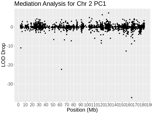
In the plot above, the position of each gene along chromosome 2 is shown on the X-axis and the LOD drop is shown on the Y-axes. Most genes don’t change the LOD score by very much. It seems that, by chance, LOD scores can vary by plus or minus 3. In this case, we are searching for genes which decrease the LOD score by the largest amount. In this case, there is one gene which reduces the LOD .
R
med_2 |>
  filter(lod_drop < -20)
OUTPUT
             gene_id base_lod  med_lod symbol    middle  lod_drop
1 ENSMUSG00000017950 97.61195 60.44990  Hnf4a 163.53986 -37.16206
2 ENSMUSG00000035000 97.61195 75.31902   Dpp4  62.37115 -22.29293
Challenge 3: Keller et al chromosome 2 hotspot candidate gene?
Look at Figure 4C in Keller et al and see which gene the selected in their mediaiton analysis.
The authors found that Hnf4a reduces the LOD more than any other gene.
Challenge 4: Look up Dpp4 in Pubmed
or Alliance Genome and see if it has any known association with type 2 diabetes or insulin metabolism.
Alliance Genome says that “Human ortholog(s) of this gene implicated in … type 2 diabetes mellitus.”
Let’s look more closely at Hnf4a. First, let’s map the expresson of Hnf4a.
R
hnf4a     <- annot[annot$symbol == "Hnf4a",]$gene_id
hnf4a_lod <- scan1(genoprobs = probs,
                  pheno     = expr_rz[,hnf4a, drop = FALSE],
                  kinship   = K,
                  addcovar  = addcovar)
plot(hnf4a_lod, map, main = "Hnf4a Genome Scan")
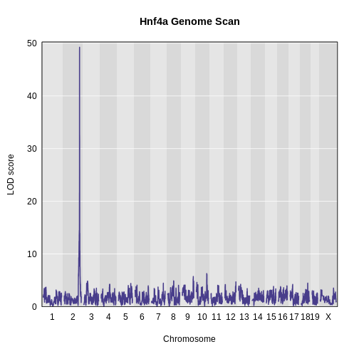
In the plot above, we can see that Hnf4a has a QTL peak on chromosome 2.
Challenge 5: Find the Hnf4a QTL peak location.
Use find_peaks() to find the position of the Hnf4a QTL peak. What kind of eQTL would you call this peak? Local or distant? How does this peak location compare with the location of the chromosome 2 eQTL hotspot?
R
find_peaks(hnf4a_lod, map = map, threshold = 8)
OUTPUT
  lodindex          lodcolumn chr      pos      lod
1        1 ENSMUSG00000017950   2 164.0224 49.25123
Hnf4a has a QTL peak on chromosome 2 at 164 Mb.
This is the same position as the chromosome 2 eQTL hotspot.
Since Hnf4a is located at 163.4 Mb and its largest eQTL is located at 164 Mb, we could call this a local eQTL.
These are the primary steps in mediation analysis. As you can see, sometimes, meditation analysis can point to a candidate gene that is plausible. It is always important to remember that there may be more than one causal gene and that causal genes may contain missense or splice SNPs which affect gene expression levels.
Interactive QTL Viewer
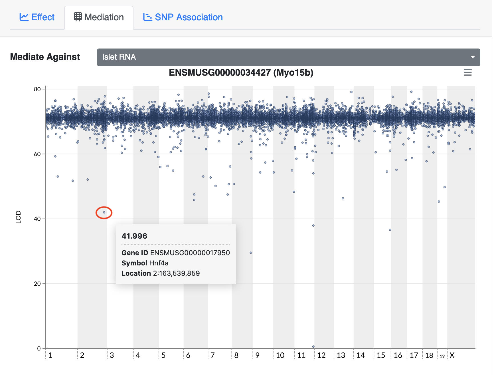
The QTL Viewer for the Attie islet data integrates mediation into exploration of the data. Below, mediation analysis identifies gene Hnf4a as the chromosome 2 gene that impacts Myo15b expression.
Challenge 6: Perform mediation at another eQTL hotspot.
Select another eQTL hotspot and perform mediation analysis.
Set “hot_chr” to one of the other eQTL hotspot locations: 5, 7, or 11
First, we look at the positions of the eQTL in this region.
R
hot_chr <- "11"
hot     <- hotspots[[hot_chr]]
plot(table(hot$qtl_pos), las = 2)
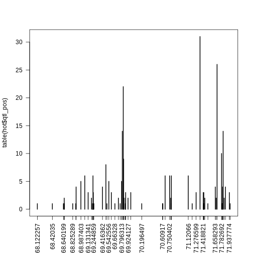
Next, we subset the genes to select ones which have eQTL at the same location. Some of the eQTL hotspots have large numbers of of genes at more than one marker. Feel free to explore different markers. Below, we sort the markers by the number of genes with eQTL at each marker so that we can select ones to pursue.
R
sort(table(hot$qtl_pos))
OUTPUT
68.122257  68.42035 68.640199 68.660126 68.825289 68.888033 68.889671  68.89049
        1         1         1         1         1         1         1         1
 69.21825 69.224642 69.231034 69.244859 69.505599  69.66328 69.768364 69.869428
        1         1         1         1         1         1         1         1
70.196497  70.60917 70.616235 70.782062 71.198629 71.422464 71.425934 71.432875
        1         1         1         1         1         1         1         1
71.510771 71.793079 71.952385 68.656091 69.198036 69.733033 69.844926 69.876397
        1         1         1         2         2         2         2         2
69.924127 70.772323 71.449172 71.675712  71.83438 69.131341  69.23423 69.592546
        2         2         2         2         2         3         3         3
69.876917 69.978753 71.276599 71.418821 71.429405 71.937774 68.892129 69.416362
        3         3         3         3         3         3         4         4
71.658293 71.803404 71.859513 68.987403 69.542556 69.796313 69.064645 69.227838
        4         4         4         5         5         5         6         6
70.661194 70.750402 70.785072  71.12066 69.484146 69.837051 71.782692 69.810287
        6         6         6         6         8         9        10        14
71.813729 69.829176 71.693132 71.354568
       14        22        26        31
Set the thresholds below to match the markers which you would like to include.
R
hot <- hot[hot$qtl_pos >= 71.3 & hot$qtl_pos <= 71.7,]
nrow(hot)
OUTPUT
[1] 75Next, we get the expression of the genes at the marker(s) we are pursuing and calculate the first pricipal component.
R
expr_hot <- expr_rz[,hot$gene_id]
hot_pca  <- princomp(expr_hot)
pc1_hot  <- hot_pca$scores[,1,drop = FALSE]
Plot the genome scan of PC1.
R
pc1_lod <- scan1(genoprobs = probs,
                 pheno     = pc1_hot,
                 kinship   = K,
                 addcovar  = addcovar)
plot_scan1(pc1_lod, map, main = paste("Chr", hot_chr))
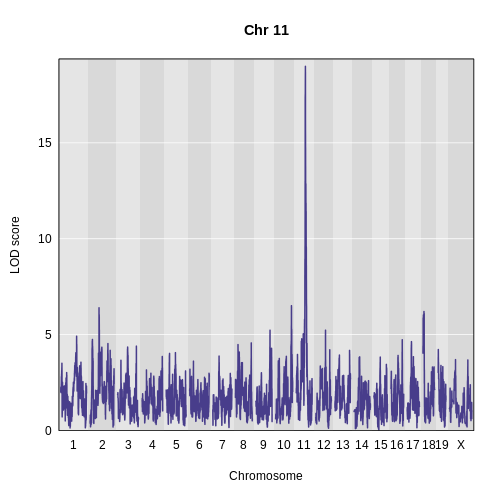
At this point, we have everything that we need to perform mediation analysis.
R
qtl_pos <- median(hot$qtl_pos)

med_hot <- mediation(qtl_chr  = hot_chr,
                     qtl_pos  = qtl_pos,
                     qtl_lod  = max(pc1_lod),
                     genoprobs = probs,
                     pheno    = pc1_hot,
                     K        = K,
                     addcovar = addcovar,
                     map      = map,
                     expr     = expr_rz,
                     annot    = annot)
WARNING
Warning in data.frame(gene_id = colnames(expr_chr), base_lod = qtl_lod, : row
names were found from a short variable and have been discarded
OUTPUT
Joining with `by = join_by(gene_id)`OUTPUT
[1] "50 of 1810 : 3.70400000000001 seconds elapsed."
[1] "100 of 1810 : 7.51500000000001 seconds elapsed."
[1] "150 of 1810 : 11.301 seconds elapsed."
[1] "200 of 1810 : 15.095 seconds elapsed."
[1] "250 of 1810 : 18.912 seconds elapsed."
[1] "300 of 1810 : 22.691 seconds elapsed."
[1] "350 of 1810 : 26.487 seconds elapsed."
[1] "400 of 1810 : 30.262 seconds elapsed."
[1] "450 of 1810 : 34.06 seconds elapsed."
[1] "500 of 1810 : 37.844 seconds elapsed."
[1] "550 of 1810 : 41.629 seconds elapsed."
[1] "600 of 1810 : 45.439 seconds elapsed."
[1] "650 of 1810 : 49.22 seconds elapsed."
[1] "700 of 1810 : 52.995 seconds elapsed."
[1] "750 of 1810 : 56.78 seconds elapsed."
[1] "800 of 1810 : 60.619 seconds elapsed."
[1] "850 of 1810 : 64.395 seconds elapsed."
[1] "900 of 1810 : 68.178 seconds elapsed."
[1] "950 of 1810 : 71.95 seconds elapsed."
[1] "1000 of 1810 : 75.736 seconds elapsed."
[1] "1050 of 1810 : 79.513 seconds elapsed."
[1] "1100 of 1810 : 83.302 seconds elapsed."
[1] "1150 of 1810 : 87.074 seconds elapsed."
[1] "1200 of 1810 : 90.865 seconds elapsed."
[1] "1250 of 1810 : 94.634 seconds elapsed."
[1] "1300 of 1810 : 98.41 seconds elapsed."
[1] "1350 of 1810 : 102.18 seconds elapsed."
[1] "1400 of 1810 : 105.978 seconds elapsed."
[1] "1450 of 1810 : 109.748 seconds elapsed."
[1] "1500 of 1810 : 113.515 seconds elapsed."
[1] "1550 of 1810 : 117.298 seconds elapsed."
[1] "1600 of 1810 : 121.092 seconds elapsed."
[1] "1650 of 1810 : 124.867 seconds elapsed."
[1] "1700 of 1810 : 128.641 seconds elapsed."
[1] "1750 of 1810 : 132.407 seconds elapsed."
[1] "1800 of 1810 : 136.192 seconds elapsed."
Now that we have completed the mediation analysis, we plot the results.
R
end  <- ceiling(max(med_hot$middle / 10))

med_hot |>
  ggplot(aes(middle, lod_drop)) +
    geom_point() +
    scale_x_continuous(breaks = 0:end * 10) +
    labs(title = str_c("Mediation Analysis for Chr ", hot_chr, " PC1"),
         x     = "Position (Mb)",
         y     = "LOD Drop") +
    theme(size = element_text(size = 20))
WARNING
Warning in plot_theme(plot): The `size` theme element is not defined in the
element hierarchy.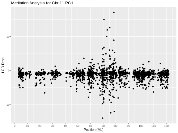
Let’s list the genes with LOD drops less than -10.
R
filter(med_hot, lod_drop < -10)
OUTPUT
             gene_id base_lod  med_lod  symbol   middle  lod_drop
1 ENSMUSG00000020846 18.98734 6.593237 Fam101b 76.02349 -12.39410
2 ENSMUSG00000069835 18.98734 5.051037    Sat2 69.62295 -13.93630
3 ENSMUSG00000072640 18.98734 6.986865   Lyrm9 78.83673 -12.00047
here are three genes with large LOD drops. In figure S7 of Keller et al, they select Sat2 as a candidate gene.
But notice that there are also gene with large LOD increases. Let’s list out the genes with LOD increases over 12.
R
filter(med_hot, lod_drop > 12)
OUTPUT
             gene_id base_lod  med_lod  symbol   middle lod_drop
1 ENSMUSG00000020829 18.98734 36.08675 Slc46a1 78.46888 17.09941
2 ENSMUSG00000040746 18.98734 33.96385  Rnf167 70.64933 14.97651
3 ENSMUSG00000045287 18.98734 31.58345 Rtn4rl1 75.23078 12.59611
There are three genes with large LOD increase. If a LOD drop means that the gene is absorbing variance and may be a causal mediator, what does a LOD increase mean?
Let’s start by looking at the allele effects of the hotspot PC1 at the QTL.
R
pr      <- pull_genoprobpos(genoprobs = probs, map = map, chr = hot_chr, pos = qtl_pos)

pc1_eff <- fit1(genoprobs = pr,
                pheno     = pc1_hot,
                kinship   = K[[hot_chr]],
                addcovar  = addcovar)
plot(1:8, pc1_eff$coef[1:8], xaxt = "n", main = "PC1", xlab = "Founder",
     ylab = "Allele Effects")
axis(side = 1, at = 1:8, labels = names(pc1_eff$coef[1:8]))
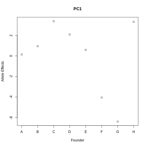
From the plot above, we can see that CAST (F) and PWK (G) have lower effects than the other founders. Remember that the sign of the PC is arbitrary, so the effects may be positive.
Next, let’s look at the allele effects of the gene with the highest LOD increase, Rnf167.
R
gene_id  <- annot[annot$symbol == "Rnf167",]$gene_id

gene_lod <- fit1(genoprobs  = pr,
                  pheno     = expr_rz[,gene_id, drop = FALSE],
                  kinship   = K[[hot_chr]],
                  addcovar  = addcovar)
plot(1:8, gene_lod$coef[1:8],  xaxt = "n", main = "Rnf167", xlab = "Founder",
     ylab = "Allele Effects")
axis(side = 1, at = 1:8, labels = names(pc1_eff$coef[1:8]))
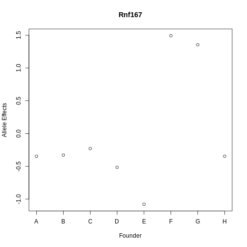
Rnf167 has allele effects which seem quite correlated with PC1. Both CAST (F) and PWK (G) have different allele effects from the other strains.
Next, let’s look at Sat2, which is the gene with the largest LOD drop.
R
gene_id  <- annot[annot$symbol == "Sat2",]$gene_id
pr       <- pull_genoprobpos(genoprobs = probs, map = map, chr = hot_chr, pos = qtl_pos)
gene_lod <- fit1(genoprobs  = pr,
                  pheno     = expr_rz[,gene_id, drop = FALSE],
                  kinship   = K[[hot_chr]],
                  addcovar  = addcovar)
plot(gene_lod$coef[1:8],xaxt = "n", main = "Sat2", xlab = "Founder",
     ylab = "Allele Effects")
axis(side = 1, at = 1:8, labels = names(pc1_eff$coef[1:8]))
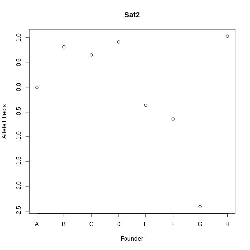
The allele effects for Sat2 appear to be less correlated, with PWK (G) having lower effects than the other strains.
Let’s look at the correlation of Sat2, Rnf167, and the hotspot PC1.
R
expr_tmp <- expr_rz[,c(annot[annot$symbol == "Sat2",]$gene_id, annot[annot$symbol == "Rnf167",]$gene_id)]
colnames(expr_tmp) <- c("Sat2", "Rnf167")
expr_tmp <- cbind(expr_tmp, pc1_hot)
cor(expr_tmp)
OUTPUT
             Sat2     Rnf167    Comp.1
Sat2    1.0000000 -0.1067984 0.5640121
Rnf167 -0.1067984  1.0000000 0.1558257
Comp.1  0.5640121  0.1558257 1.0000000
Both genes have almost identical correlation (0.41) with PC1, but are not strongly correlated with each other (-0.1).
Let’s look at the relationship between the correlation between PC1 and all of the genes on chromosome 11.
R
expr_11 <- expr_rz[,annot[annot$chr == '11',]$gene_id]
cor_11  <- cor(pc1_hot, expr_11)
WARNING
Warning in cor(pc1_hot, expr_11): the standard deviation is zeroR
plot(med_hot$lod_drop, cor_11, xlab = "LOD Drop", ylab = "Correlation")
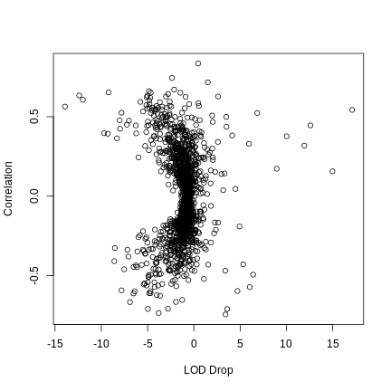
There seems to be a relationship between the absolute LOD drop and the correlation between the gene and PC1.
Mediation analysis is one way of identifying candidate genes under QTL peaks. In this episode, we have focused on eQTL hotspots, but you could do this with physiological phenotypes as well.
- Mediation analysis investigates an intermediary between an independent variable and its effect on a dependent variable.
- Mediation analysis is used in high-throughput genomics studies to identify molecular phenotypes, such as gene expression or methylation traits, that mediate the effect of genetic variation on disease phenotypes or other outcomes of interest.
