Mapping A Single Gene Expression Trait

Overview

Teaching: 30 min
Exercises: 30 min

Questions

• How do I map one gene expression trait?

Objectives

• QTL mapping of an expression data set

In this tutorial, we are going to use the gene expression data as our phenotype to map QTLs. That is, we are looking to find any QTLs (cis or trans) that are responsible for variation in gene expression across samples.

We are using the same directory as our previous tutorial, which you can check by typing getwd() in the Console. If you are not in the correct directory, type in setwd("code") in the console or Session -> Set Working Directory -> Choose Directory in the RStudio menu to set your working directory to the main directory.

If you have started a new R session, you will need to load the libraries again. If you haven’t, the libraries listed below are already loaded.

Load Libraries

library(tidyverse)
library(knitr)
library(broom)
library(qtl2)

Load Data

In this lesson, we are loading in gene expression data for 21,771 genes: attie_DO500_expr.datasets.RData that includes normalised and raw gene expression data. dataset.islet.rnaseq is the dataset you can download directly from Dryad. Again, if you are using the same R session, you will not need to the load the mapping, phenotypes and genotype probabilities data, again.

# expression data
load("../data/attie_DO500_expr.datasets.RData")

# data from paper
load("../data/dataset.islet.rnaseq.RData")

# phenotypes
load("../data/attie_DO500_clinical.phenotypes.RData")

# mapping data
load("../data/attie_DO500_mapping.data.RData")

# genotype probabilities
probs = readRDS("../data/attie_DO500_genoprobs_v5.rds")

Expression Data

Raw gene expression counts are in the counts data object. These counts have been normalised and saved in the norm data object. More information is about normalisation is here.

To view the contents of either one of these data , click the table on the right hand side either norm or counts in the Environment tab. If you type in names(counts), you will see the names all start with ENSMUSG. These are Ensembl IDs. If we want to see which gene these IDs correspond to, type in dataset.islet.rnaseq$annots, which gives information about each gene, including ensemble id, gene symbol as well as start & stop location of the gene and chromsome on which the gene lies.

Because we are working with the insulin tAUC phenotype, let’s map the expression counts for Hnf1b which is known to influence this phenotype is these data. First, we need to find the Ensembl ID for this gene:

dataset.islet.rnaseq$annots[dataset.islet.rnaseq$annots$symbol == "Hnf1b",]

                              gene_id symbol chr    start      end strand
ENSMUSG00000020679 ENSMUSG00000020679  Hnf1b  11 83.85006 83.90592      1
                     middle nearest.marker.id        biotype       module
ENSMUSG00000020679 83.87799       11_84097611 protein_coding midnightblue
                   hotspot
ENSMUSG00000020679    <NA>

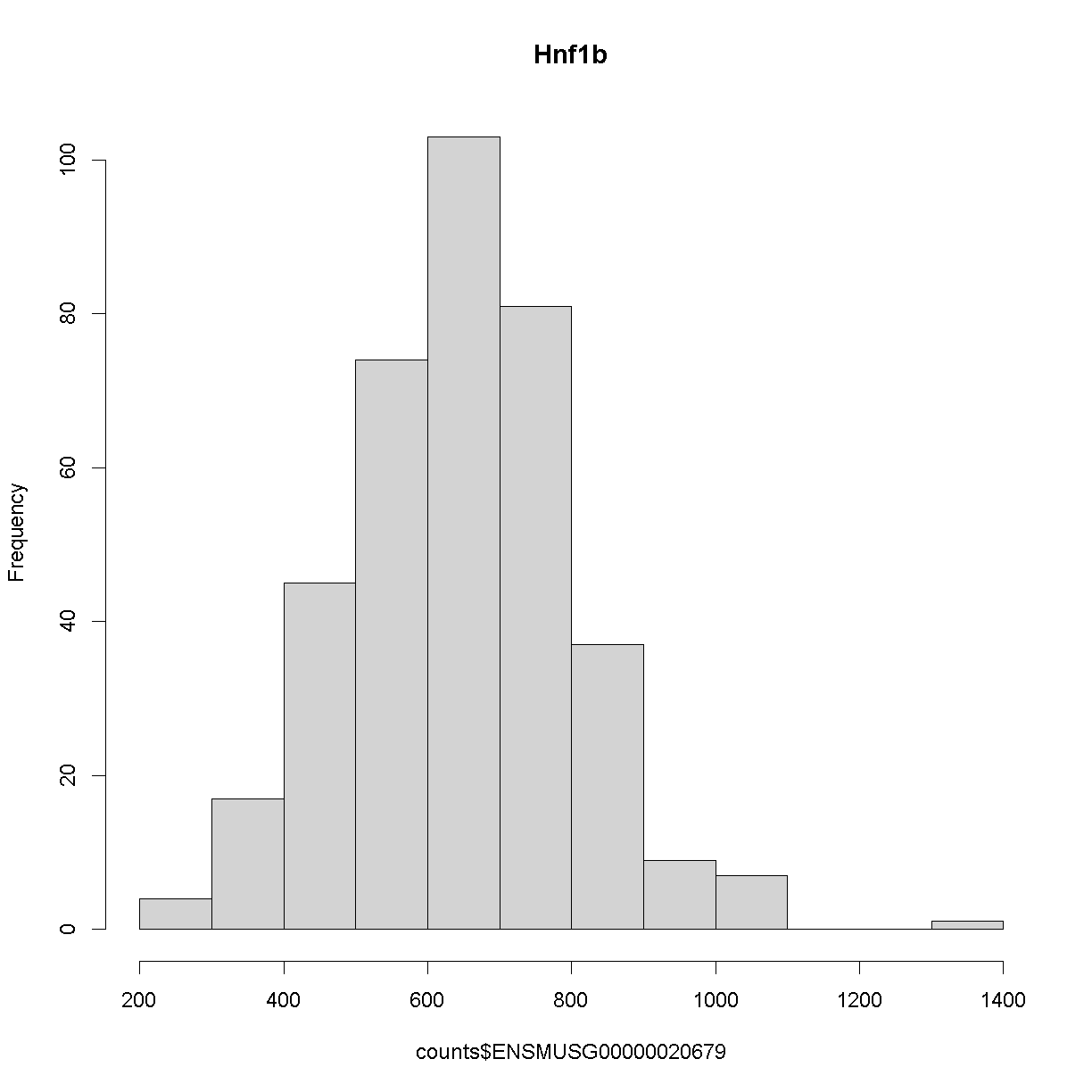
We can see that the ensembl ID of Hnf1b is ENSMUSG00000020679. If we check the distribution for Hnf1b expression data between the raw and normalised data, we can see there distribution has been corrected. Here is the distribution of the raw counts:

hist(counts$ENSMUSG00000020679, main = "Hnf1b")

and here is the distribution of the normalised counts:

hist(norm$ENSMUSG00000020679, main = "Hnf1b")

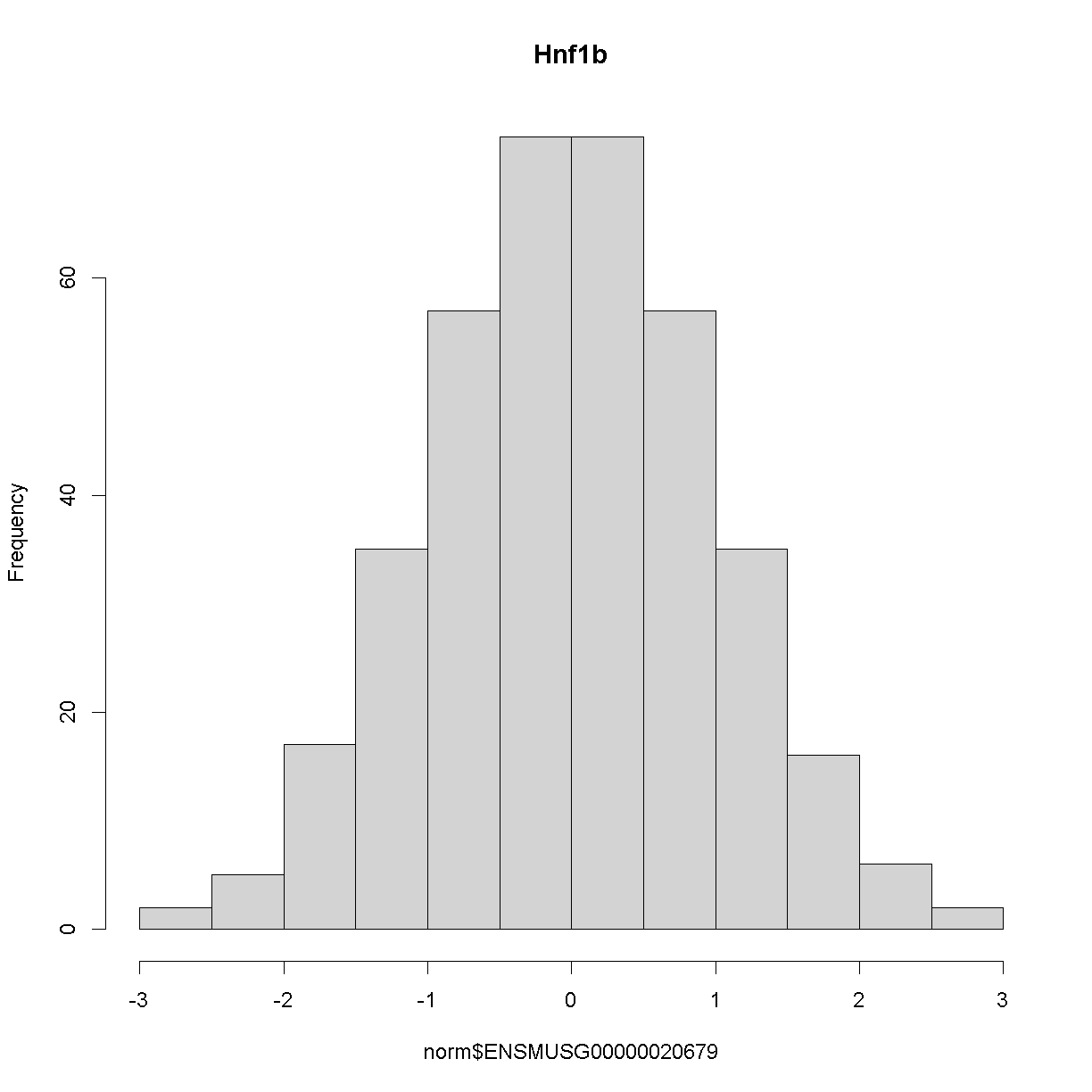
The histogram indicates that distribution of these counts are normalised.

The Marker Map

We are using the same marker map as in the previous lesson

Genotype probabilities

We have explored this earlier in th previous lesson. But, as a reminder, we have already calculated genotype probabilities which we loaded above called probs. This contains the 8 state genotype probabilities using the 69k grid map of the same 500 DO mice that also have clinical phenotypes.

Kinship Matrix

We have explored the kinship matrix in the previous lesson. It has already been calculated and loaded in above.

Covariates

Now let’s add the necessary covariates. For Hnf1b expression data, let’s see which covariates are significant.

###merging covariate data and expression data to test for sex, wave and diet_days.

cov.counts <- merge(covar, norm, by=c("row.names"), sort=F)

#testing covairates on expression data

tmp = cov.counts %>%
        dplyr::select(mouse, sex, DOwave, diet_days, ENSMUSG00000020679) %>%
        gather(expression, value, -mouse, -sex, -DOwave, -diet_days) %>%
        group_by(expression) %>%
        nest()
mod_fxn = function(df) {
  lm(value ~ sex + DOwave + diet_days, data = df)
}
tmp = tmp %>%
  mutate(model = map(data, mod_fxn)) %>%
  mutate(summ = map(model, tidy)) %>%
  unnest(summ) 
#  kable(tmp, caption = "Effects of Sex, Wave & Diet Days on Expression")

tmp

# A tibble: 4 x 8
# Groups:   expression [1]
  expression         data     model  term      estimate std.e~1 stati~2  p.value
  <chr>              <list>   <list> <chr>        <dbl>   <dbl>   <dbl>    <dbl>
1 ENSMUSG00000020679 <tibble> <lm>   (Interce~ -1.70    0.506     -3.36 8.72e- 4
2 ENSMUSG00000020679 <tibble> <lm>   sexM      -0.199   0.0824    -2.42 1.60e- 2
3 ENSMUSG00000020679 <tibble> <lm>   DOwave     0.510   0.0370    13.8  3.73e-35
4 ENSMUSG00000020679 <tibble> <lm>   diet_days  0.00403 0.00386    1.04 2.97e- 1
# ... with abbreviated variable names 1: std.error, 2: statistic

tmp %>%
  filter(term != "(Intercept)") %>%
  mutate(neg.log.p = -log10(p.value)) %>%
  ggplot(aes(term, neg.log.p)) +
    geom_point() +
    facet_wrap(~expression) +
    labs(title = "Significance of Sex, Wave & Diet Days on Expression") +
    theme(axis.text.x = element_text(angle = 90, hjust = 1, vjust = 0.5)) +
rm(tmp)

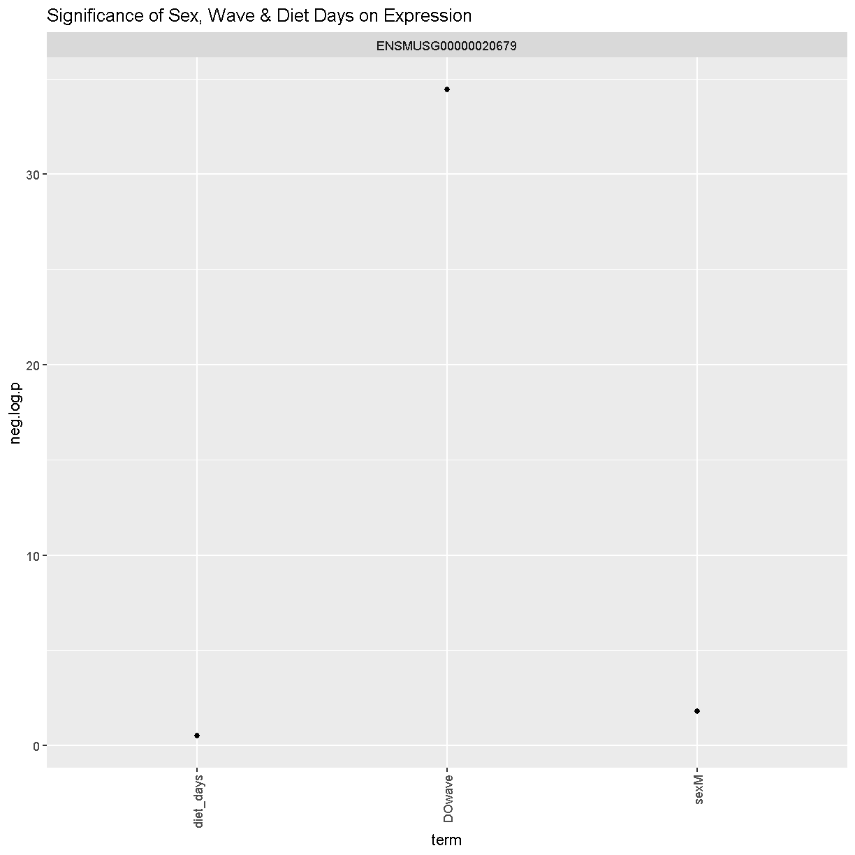
We can see that sex and DOwave are significant. Here DOwave is the group or batch number as not all mice were submitted for genotyping at the same time. Because of this, we now have to correct for it. Considering the paper included the covariate, diet_days, we will include that as well.

# convert sex and DO wave (batch) to factors
pheno_clin$sex = factor(pheno_clin$sex)
pheno_clin$DOwave = factor(pheno_clin$DOwave)
pheno_clin$diet_days = factor(pheno_clin$DOwave)

covar = model.matrix(~sex + DOwave + diet_days, data = pheno_clin)[,-1]

Performing a genome scan

[Permutations]

First, we need to work out the signifcance level. Let’s find the signifance level for 0.1, 0.05 and 0.01.

operm <- scan1perm(genoprobs = probs, 
                   pheno = norm[,"ENSMUSG00000020679", drop = FALSE], 
                   addcovar=covar,
                   n_perm=1000)

Note DO NOT RUN THIS (it will take too long). Instead, I have run it earlier and will load it in here. We will also perform a summary to find the summary level for 0.1, 0.05 and 0.01

load("../data/operm_ENSMUSG00000020679_1000.Rdata")

summary(operm,alpha=c(0.1, 0.05, 0.01))

LOD thresholds (1000 permutations)
     ENSMUSG00000020679
0.1                7.29
0.05               7.73
0.01               8.30

Genome Scan

qtl = scan1(genoprobs = probs, 
            pheno = norm[,"ENSMUSG00000020679", drop = FALSE], 
            kinship = K, 
            addcovar = covar)

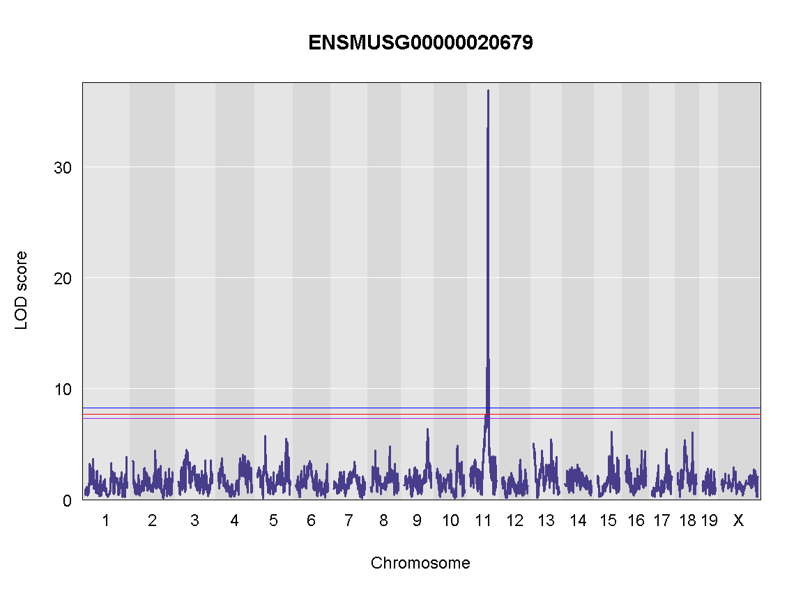
Next, we plot the genome scan.

plot_scan1(x = qtl, 
           map = map, 
           lodcolumn = "ENSMUSG00000020679",
           main = colnames(qtl))
           add_threshold(map,  summary(operm, alpha=0.1), col = 'purple')
           add_threshold(map,  summary(operm, alpha=0.05), col = 'red')
           add_threshold(map,  summary(operm, alpha=0.01), col = 'blue')

Finding LOD peaks

Let’s find LOD peaks

lod_threshold = summary(operm, alpha=0.01)
peaks = find_peaks(scan1_output = qtl, 
                   map = map, 
                   threshold = lod_threshold, 
                   peakdrop = 4, prob = 0.95)
kable(peaks %>% 
        dplyr::select(-lodindex) %>% 
        arrange(chr, pos), caption = "Phenotype QTL Peaks with LOD >= 6")

Table: Phenotype QTL Peaks with LOD >= 6

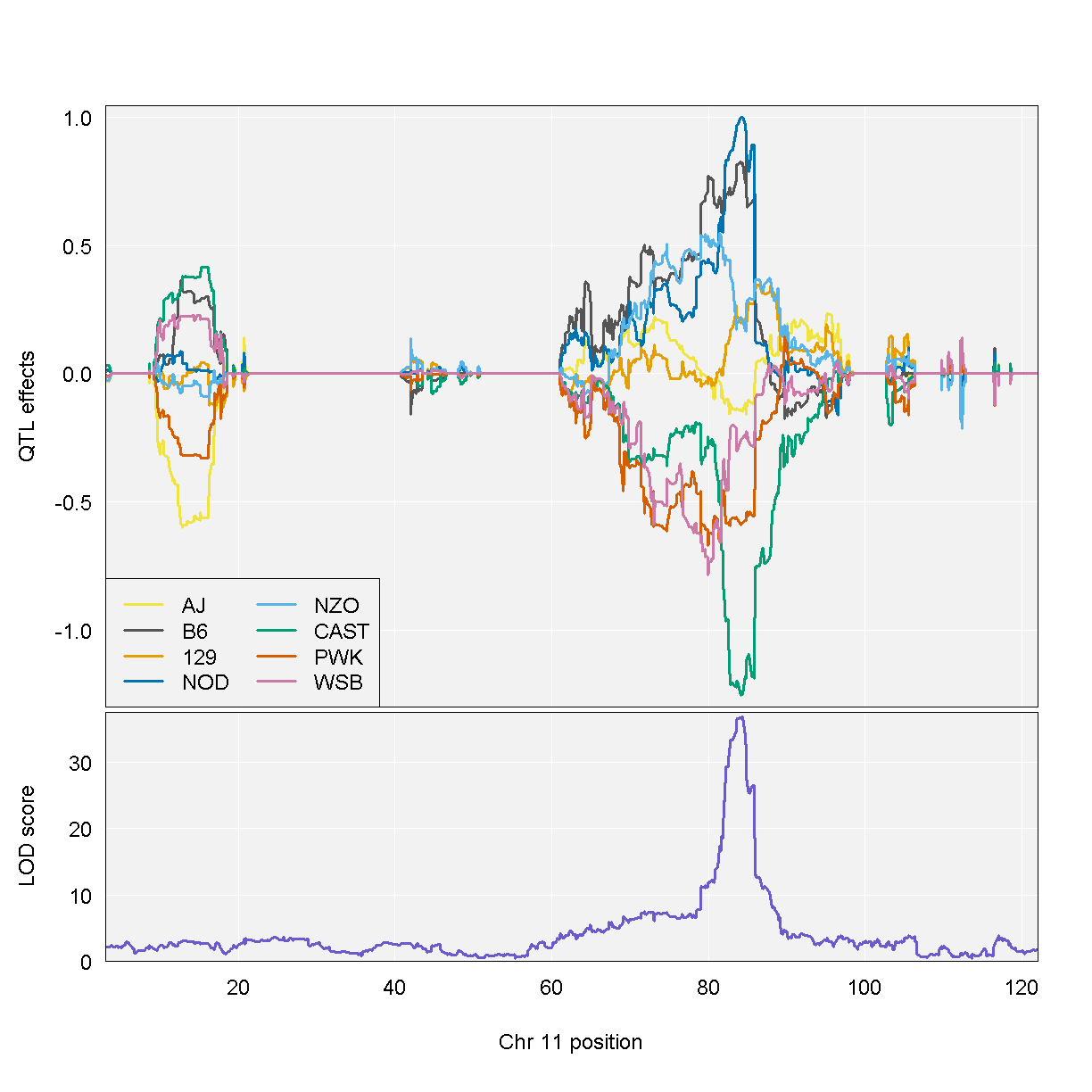
QTL effects

blup <- scan1blup(genoprobs=probs[,peaks$chr[1]], 
                  norm[,peaks$lodcolumn[1], drop=FALSE])

plot_coefCC(blup, 
       map=map, 
       columns=1:8,
       bgcolor="gray95", 
       legend="bottomleft",
       scan1_output = qtl )

Challenge

Now choose another gene expression trait in norm data object and perform the same steps.
1). Check the distribution of the raw counts and normalised counts 2). Are there any sex, batch, diet effects?
3). Run a genome scan with the genotype probabilities and kinship provided.
4). Plot the genome scan for this gene.
5). Find the peaks above LOD score of 6.

Solution

Replace <ensembl id> with your choice of gene expression trait

#1).

hist(pheno_clin$<ensembl id>)

pheno_clin$<ensembl id>_log <- log(pheno_clin$<ensembl id>)

hist(pheno_clin$<ensembl id>_log)


#2).

tmp = pheno_clin %>%
        dplyr::select(mouse, sex, DOwave, diet_days, <ensembl id>) %>%
        gather(expression, value, -mouse, -sex, -DOwave, -diet_days) %>%
        group_by(expression) %>%
        nest()
mod_fxn = function(df) {
  lm(value ~ sex + DOwave + diet_days, data = df)
}
tmp = tmp %>%
  mutate(model = map(data, mod_fxn)) %>%
  mutate(summ = map(model, tidy)) %>%
  unnest(summ) 

tmp

tmp %>%
  filter(term != "(Intercept)") %>%
  mutate(neg.log.p = -log10(p.value)) %>%
  ggplot(aes(term, neg.log.p)) +
    geom_point() +
    facet_wrap(~expression) +
    labs(title = "Significance of Sex, Wave & Diet Days on Phenotypes") +
    theme(axis.text.x = element_text(angle = 90, hjust = 1, vjust = 0.5)) +
rm(tmp)

#3).

qtl = scan1(genoprobs = probs, 
           pheno = pheno_clin[,"<ensembl id>", drop = FALSE], 
        kinship = K, 
        addcovar = covar)

#4).

plot_scan1(x = qtl, map = map, lodcolumn = "<ensembl id>")
abline(h = 6, col = 2, lwd = 2)

#5). 

peaks = find_peaks(scan1_output = qtl, map = map, 
               threshold = lod_threshold, 
               peakdrop = 4, 
               prob = 0.95)

Key Points

• To run a QTL analysis for expression data