Creating A Transcriptome Map

Overview

Teaching: 30 min
Exercises: 30 min

Questions

• How do I create and interpret a transcriptome map?

Objectives

• Describe a transcriptome map.

• Interpret a transcriptome map.

Load Libraries

library(tidyverse)
library(qtl2)
library(qtl2convert)
library(RColorBrewer)
library(qtl2ggplot)

source("../code/gg_transcriptome_map.R")

Load Data

Load in the LOD peaks over 6 from previous lesson.

# REad in the LOD peaks from the previous lesson.
lod_summary <- read.csv("../results/gene.norm_qtl_peaks_cis.trans.csv")

In order to use the ggtmap function, we need to provide specific column names. These are documented in the “gg_transcriptome_map.R” file in the code directory of this workshop. The required column names are:

• data: data.frame (or tibble) with the following columns:
  • ensembl: (required) character string containing the Ensembl gene ID.
  • qtl_chr: (required) character string containing QTL chromsome.
  • qtl_pos: (required) floating point number containing the QTL position in Mb.
  • qtl_lod: (optional) floating point number containing the LOD score.
  • gene_chr: (optional) character string containing transcript chromosome.
  • gene_start: (optional) character string containing transcript start postion in Mb.
  • gene_end: (optional) character string containing transcript end position in Mb.

# Get gene positions.
ensembl <- get_ensembl_genes()
df <- data.frame(ensembl    = ensembl$gene_id, 
                 gene_chr   = seqnames(ensembl), 
                 gene_start = start(ensembl) * 1e-6, 
                 gene_end   = end(ensembl)   * 1e-6,
                 stringsAsFactors = F)

lod_summary <- lod_summary %>% 
                 rename(lodcolumn = "ensembl",
                        chr       = "qtl_chr",
                        pos       = "qtl_pos",
                        lod       = "qtl_lod") %>% 
                 left_join(df, by = "ensembl") %>% 
                 mutate(marker.id = str_c(qtl_chr, qtl_pos * 1e6, sep = "_"),
                        gene_chr  = factor(gene_chr, levels = c(1:19, "X")),
                        qtl_chr   = factor(qtl_chr, levels = c(1:19, "X")))

rm(df)

Some of the genes will have a QTL in the same location as the gene and others will have a QTL on a chromosome where the gene is not located.

Challenge

a. What do we call eQTL that are co-colocated with the gene? b. What do we call eQTL that are located on a different chromosome than the gene?

Solution

a. A cis-eQTL is an eQTL that is co-colocated with the gene. b. A trans-eQTL is an eQTL that is located on a chromosome other than the gene that was mapped.

We can tabluate the number of cis- and trans-eQTL that we have and add this to our QTL summary table. A cis-eQTL occurs when the QTL peaks is directly over the gene position. But what if it is 2 Mb away? Or 10 Mb? It’s possible that a gene may have a trans eQTL on the same chromosome if the QTL is “far enough” from the gene. We have selected 4 Mb as a good rule of thumb.

lod_summary <- lod_summary %>% 
                     mutate(cis = if_else(qtl_chr == gene_chr & abs(gene_start - qtl_pos) < 4, "cis", "trans"))
count(lod_summary, cis)

    cis  n
1   cis 33
2 trans 55

Plot Transcriptome Map

ggtmap(data = lod_summary %>% filter(qtl_lod >= 7.18), cis.points = TRUE, cis.radius = 4)

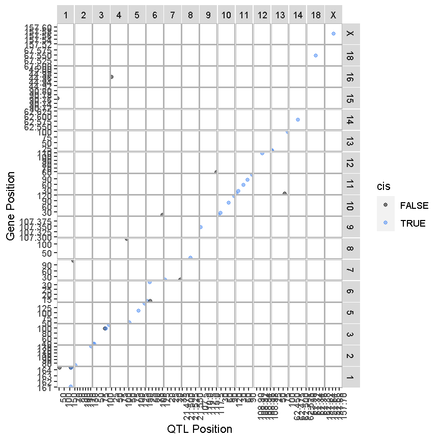
The plot above is called a “Transcriptome Map” because it shows the postions of the genes (or transcripts) and their corresponding QTL. The QTL position is shown on the X-axis and the gene position is shown on the Y-axis. The chromosomes are listed along the top and right of the plot. What type of QTL are the genes with QTL that are located along the diagonal?

Key Points

• Transcriptome maps aid in understanding gene expression regulation.