Loading data into R

Overview

Teaching: 40 min
Exercises: 20 min

Questions

How do I load data into R?

Objectives

Install and load packages.

Locate files in a file and directory hierarchy.

Read in data from a .csv file into a data frame.

Describe a data frame.

Subset a data frame.

Loading data into R

Loading data into R is the first step!

First we need to load up a package to make loading data sets easier. We will be using the tidyverse set of packages for all of our data processing needs in R. This is not the only way you can process data in R, but from experience, it seems to be the easier way to learn R due to its consistency, community, and learning materials.

"Tidyverse Celestial" by Allison Horst. "tidyverse" hex sticker in space surrounded by other tidyverse package hex logos.

We first will load up the tidyverse packages using the library function.

library(tidyverse)

── Attaching packages ──────────────────────────────────────────────────────────────────────────────────────────────────────────────────────────────────────── tidyverse 1.3.0 ──

✔ ggplot2 3.3.5     ✔ purrr   0.3.4
✔ tibble  3.1.4     ✔ dplyr   1.0.7
✔ tidyr   1.1.3     ✔ stringr 1.4.0
✔ readr   1.4.0     ✔ forcats 0.5.1

── Conflicts ─────────────────────────────────────────────────────────────────────────────────────────────────────────────────────────────────────────── tidyverse_conflicts() ──
✖ dplyr::filter() masks stats::filter()
✖ dplyr::lag()    masks stats::lag()

The first time you load up the tidyverse library, there will be some output that lists the packages tidyverse loads, along with any functions that share the same name as other functions (i.e., conflicts). As long as you are mindful about starting a new RStudio session before you work, you can ignore this output for now.

Now we can use all the functions within the Tidyverse to do our data processing. If you are following along and you run a piece of code and end up with an could not find function error, make sure you typed library(tidyverse) correctly and executed the line of code.

Find your files

Let the below figures represent a ds4biomed folder on your Desktop on Windows and Mac, respectively.

:::{.row} :::{.column}

C:\
  |- Users\
    |- Daniel\
      |- Desktop\
        |- ds4biomed\
         |- data\
         |    |- medicaldata_tumorgrowth.csv
         |- output\
         |- 01-load_data.R
         |- README.md
         |- ds4biomed.Rproj

:::

:::{.column}

/
  |- Users/
    |- Daniel/
      |- Desktop/
        |- ds4biomed/
          |- data/
          |    |- medicaldata_tumorgrowth.csv
          |- output/
          |- 01-load_data.R
          |- README.md
          |- ds4biomed.Rproj

::: :::

Suppose we are “in” the ds4biomed folder, where we can see the data and output folders along with the 01-load_data.R, README.md, and ds4biomed.Rproj files.

We can reference our medicaldata_tumorgrowth.csv file inside the data folder as: data/medicaldata_tumorgrowth.csv. That is, we can use the backslash, / to move into folders. We can write data/medicaldata_tumorgrowth.csv because we are “starting from” the ds4biomed folder. This is called a relative path because the location of the csv file is relative to the ds4biomed starting point (aka working directory). If we want to refer to any arbitrary filer or folder on the computer, we can specify the full path of the file. The full path will start with a drive letter on windows, C:\Users\Daniel\Desktop\ds4biomed\data\medicaldata_tumorgrowth.csv, and a / on a Mac, /Users/Daniel/Desktop/ds4biomed/data/medicaldata_tumorgrowth.csv.

Suppose we create an analysis folder for our 01-load_data.R script so that our folder structure looks like this (only the mac version is shown in the example below):

/
  |- Users/
    |- Daniel/
      |- Desktop/
        |- ds4biomed/
          |- data/
          |    |- medicaldata_tumorgrowth.csv
          |- output/
          |- analysis
          |    |- 01-load_data.R
          |- README.md
          |- ds4biomed.Rproj

Now, if our working directory is now in the analysis folder, we need a way to reference one folder up to the ds4biomed folder and then back down to the data folder. The way we can relatively reference the previous folder is with 2 dots, .., ../data/medicaldata_tumorgrowth.csv

/
  |- Users/
    |- Daniel/
      |- projects/
        |-chart_review/
        |    |- data/
        |    |    |- patients.csv
        |    |- analysis/
        |         |- demographics.R # you are working here
        |- rct_m22-0305
             |- data/
                  |- patients.csv

Exercise 1

Refer to the example folder structure above where we have a chart_review/ and rct_m22-0305/ folder in our projects/ folder. Let’s say we are currently in the chart_review/analysis/ folder, working on our demographics.R as denoted by the #.

Write the relative path to the patients.csv file in the rct_m22-0305/ folder.

Write the absolute path to the patients.csv file in the chart_review/ folder.

Solution

Assuming that we are located in the chart_review/analysis/ folder, the relative path to the patients.csv file located in the rct_m22-0305 folder is
../../rct_m22-0305/data/patients.csv on a Mac. One set of ../ brings us up a level to the chart_review folder, while the second set of ../ brings us up a level to the projects folder. Then we can descend into the rct_m22-0305 folder followed by the data folder.

The absolute path to the patients.csv file in the chart_review/ folder is
/Users/Daniel/projects/chart_review/data/patients.csv on a Mac
and
C:\Users\Daniel\projects\chart_review\data\patients.csv on Windows.

Paths in Windows

When you are looking at file paths in the Windows Explorer, you will notice that all Windows paths will use the backslash, \, instead of the forward slash, / to refer to files. In a lot of programming languages, including R, the \ is a special character, so if you want to use \ for file paths in Windows, you will have to use 2 backslashes, e.g., ..\\data\\patients.csv\\. However, you can still use the regular / in Windows to refer to folders just like other operating systems.

Set your working directory

So far, we have been talking about a “starting point” or “working directory”, when we have been referring to files around our computer. In order to quickly and reliably set your working directory, we use RStudio Projects.

Reading text files (CSV)

Now that we know how to find our files, let’s load up our first data set. Make sure you are in your analysis folder by typing getwd() in the Console. If you need to move into the analysis folder you can use
Session → Set Working Directory → Choose Directory. When trying to type in a file path, you can hit the <TAB> key to autocomplete the files. This will help you with a lot of potential spelling mistakes.

read_csv("../data/medicaldata_tumorgrowth.csv")

── Column specification ─────────────────────────────────────────────────────────────────────────────────────────────────────────────────────────────────────────────────────────
cols(
  Grp = col_character(),
  Group = col_double(),
  ID = col_double(),
  Day = col_double(),
  Size = col_double()
)

# A tibble: 574 × 5
   Grp   Group    ID   Day   Size
   <chr> <dbl> <dbl> <dbl>  <dbl>
1.CTR     1   101     0   41.8
1.CTR     1   101     3   85  
1.CTR     1   101     4  114  
1.CTR     1   101     5  162. 
1.CTR     1   101     6  178. 
1.CTR     1   101     7  325  
1.CTR     1   101    10  624. 
1.CTR     1   101    11  648. 
1.CTR     1   101    12  836. 
1.CTR     1   101    13 1030. 
# … with 564 more rows

Debug help:

If the above code returns a could not find function "read_csv" make sure you have loaded up the proper library with library(tidyverse)
If the above code returns a does not exist in current working directory, make sure the working directory it lists is your expected “starting point” (i.e., working directory), and make sure the file path is spelled correctly.

read_csv will show us the columns that were read in, as well as the data type of that column (e.g., character, double – a number).

The dataset we loaded is a modified version of the tumorgrowth dataset contributed by Dr. Constantine Daskalakis at Thomas Jefferson University The data show the treatment group for a particular sample and its tumor size ($mm^3$) over time (days).

Cells from a human glioma cell line were implanted in the flank of n=37 nude mice and a subcutaneous tumor (xenograft) was allowed to grow. When a tumor grew to around 40-60 $mm^3$, the animal was assigned to one of 4 experimental groups (day 0):
1) Control (CTR, n=8);
2) Drug only (D, n=10);
3) Radiation only (R, n=10); and
4) Drug + Radiation (D+R, n=9).
The main outcome in xenograft experiments is the size (volume) of the tumor over time. In this study, tumor size was typically measured every work day (excluding weekends and holidays, and occasional skipped days) for up to 4 weeks. An animal was euthanized if it appeared distressed or moribund, or when its tumor grew to about 2 cm3. The study’s two main scientific aims were to assess whether:
a. The drug has an effect on tumor growth.
b. The administration of the drug before radiation enhances the effect of the latter on tumor growth.

You can read more about the dataset and study in “Mixed-Effects Modeling of Tumor Growth in Animal Xenograft Experiments”

What do you predict?

1). What do you predict were the outcomes of this tumor growth study? Did the drug have an effect? Did the drug enhance the effect of radiation on tumor growth? Which experimental group generated the largest tumor sizes? the smallest?
2). How can we determine if there is a significant difference between experimental groups with the largest and smallest tumor sizes? How can we determine whether the drug had an effect on radiation? 3). How might you check your answer to number 2 above?

Solution

Making predictions about the results of a study motivates the need for statistical methods. If all results were predictable, we would not need either data or statistics. There are no right or wrong answers here - the purpose is to think statistically! For question 2, t-tests and visualizations can help to determine whether there is a difference in means or an effect between treatment groups.

Loading a data set is great, but we need a convenient way to refer to the data set. We don’t want to re-load the data set every time we want to perform an action on it. We can take this loaded data set and assign it to a variable. We can do this with the assignment operator, <-. Note the way it is typed, a less than symbol (<) followed immediately by the dash (-) without any spaces in between. The right side of the assignment operator, <-, will be executed and then assigned to the variable on the left.

tumor <- read_csv("../data/medicaldata_tumorgrowth.csv")

── Column specification ─────────────────────────────────────────────────────────────────────────────────────────────────────────────────────────────────────────────────────────
cols(
  Grp = col_character(),
  Group = col_double(),
  ID = col_double(),
  Day = col_double(),
  Size = col_double()
)

Notice this time we no longer see the dataset being printed. The “Environment” tab in the RStudio panel will now have an entry for the variable you used. Clicking on the right data set icon will open a view of your dataset, clicking on the arrow will show you the column-by-column text representation (technically it’s called the structure).

To look at our dataset we can execute just the variable we assigned the dataset to.

tumor

# A tibble: 574 × 5
   Grp   Group    ID   Day   Size
   <chr> <dbl> <dbl> <dbl>  <dbl>
1.CTR     1   101     0   41.8
1.CTR     1   101     3   85  
1.CTR     1   101     4  114  
1.CTR     1   101     5  162. 
1.CTR     1   101     6  178. 
1.CTR     1   101     7  325  
1.CTR     1   101    10  624. 
1.CTR     1   101    11  648. 
1.CTR     1   101    12  836. 
1.CTR     1   101    13 1030. 
# … with 564 more rows

This tabular dataset that has now been loaded into R is called a data frame object (or simply dataframe), the tidyverse uses a tibble. For the most part, a data.frame object will behave like a tibble object.

What are data frames?

When we loaded the data into R, it got stored as an object of class tibble, which is a special kind of data frame (the difference is not important for our purposes, but you can learn more about tibbles here). Data frames are the de facto data structure for most tabular data, and what we use for statistics and plotting. Data frames can be created by hand, but most commonly they are generated by functions like read_csv(); in other words, when importing spreadsheets from your hard drive or the web.

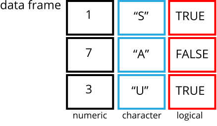
A data frame is the representation of data in the format of a table where the columns are vectors that all have the same length. Because columns are vectors, each column must contain a single type of data (e.g., characters, integers, factors). For example, here is a figure depicting a data frame comprising a numeric, a character, and a logical vector.

example data frame We can see this also when inspecting the structure of a data frame with the function str():

str(tumor)

spec_tbl_df [574 × 5] (S3: spec_tbl_df/tbl_df/tbl/data.frame)
 $ Grp  : chr [1:574] "1.CTR" "1.CTR" "1.CTR" "1.CTR" ...
 $ Group: num [1:574] 1 1 1 1 1 1 1 1 1 1 ...
 $ ID   : num [1:574] 101 101 101 101 101 101 101 101 101 101 ...
 $ Day  : num [1:574] 0 3 4 5 6 7 10 11 12 13 ...
 $ Size : num [1:574] 41.8 85 114 162.3 178.3 ...
 - attr(*, "spec")=
  .. cols(
  ..   Grp = col_character(),
  ..   Group = col_double(),
  ..   ID = col_double(),
  ..   Day = col_double(),
  ..   Size = col_double()
  .. )

head(tumor)

# A tibble: 6 × 5
  Grp   Group    ID   Day  Size
  <chr> <dbl> <dbl> <dbl> <dbl>
1 1.CTR     1   101     0  41.8
2 1.CTR     1   101     3  85  
3 1.CTR     1   101     4 114  
4 1.CTR     1   101     5 162. 
5 1.CTR     1   101     6 178. 
6 1.CTR     1   101     7 325  

Inspecting data frames

We already saw how the functions head() and str() can be useful to check the content and the structure of a data frame. Here is a non-exhaustive list of functions to get a sense of the content/structure of the data. Let’s try them out!

Size:
- dim(tumor) - returns a vector with the number of rows in the first element, and the number of columns as the second element (the dimensions of the object)
- nrow(tumor) - returns the number of rows
- ncol(tumor) - returns the number of columns
Content:
- head(tumor) - shows the first 6 rows
- tail(tumor) - shows the last 6 rows
Names:
- names(tumor) - returns the column names (synonym of colnames() for data.frame objects)
- rownames(tumor) - returns the row names
Summary:
- str(tumor) - structure of the object and information about the class, length and content of each column
- summary(tumor) - summary statistics for each column

Note: most of these functions are “generic”, they can be used on other types of objects besides data.frame.

Exercise

Based on the output of str(tumor), can you answer the following questions?

What is the class of the object tumor?

How many rows and how many columns are in this object?
Solution
str(tumor)  
spec_tbl_df [574 × 5] (S3: spec_tbl_df/tbl_df/tbl/data.frame)
 $ Grp  : chr [1:574] "1.CTR" "1.CTR" "1.CTR" "1.CTR" ...
 $ Group: num [1:574] 1 1 1 1 1 1 1 1 1 1 ...
 $ ID   : num [1:574] 101 101 101 101 101 101 101 101 101 101 ...
 $ Day  : num [1:574] 0 3 4 5 6 7 10 11 12 13 ...
 $ Size : num [1:574] 41.8 85 114 162.3 178.3 ...
 - attr(*, "spec")=
  .. cols(
  ..   Grp = col_character(),
  ..   Group = col_double(),
  ..   ID = col_double(),
  ..   Day = col_double(),
  ..   Size = col_double()
  .. )
class: data frame

how many rows: 574, how many columns: 5

Indexing and subsetting data frames

Our data frame has rows and columns (it has 2 dimensions), if we want to extract some specific data from it, we need to specify the “coordinates” we want from it. Row numbers come first, followed by column numbers. However, note that different ways of specifying these coordinates lead to results with different classes.

We can extract specific values by specifying row and column indices in the format: data_frame[row_index, column_index] For instance, to extract the first row and column from tumor:

tumor[1, 1]

# A tibble: 1 × 1
  Grp  
  <chr>
1 1.CTR

First row, fifth column:

tumor[1, 5]   

# A tibble: 1 × 1
   Size
  <dbl>
1  41.8

We can also use shortcuts to select a number of rows or columns at once To select all columns, leave the column index blank For instance, to select all columns for the first row:

tumor[1, ]

# A tibble: 1 × 5
  Grp   Group    ID   Day  Size
  <chr> <dbl> <dbl> <dbl> <dbl>
1 1.CTR     1   101     0  41.8

The same shortcut works for rows – To select the first column across all rows:

tumor[, 1]

# A tibble: 574 × 1
   Grp  
   <chr>
1.CTR
1.CTR
1.CTR
1.CTR
1.CTR
1.CTR
1.CTR
1.CTR
1.CTR
1.CTR
# … with 564 more rows

An even shorter way to select first column across all rows:

tumor[1] # No comma! 

# A tibble: 574 × 1
   Grp  
   <chr>
1.CTR
1.CTR
1.CTR
1.CTR
1.CTR
1.CTR
1.CTR
1.CTR
1.CTR
1.CTR
# … with 564 more rows

To select multiple rows or columns, use vectors! To select the first three rows of the 4th and 5th column

tumor[c(1, 2, 3), c(4, 5)] 

# A tibble: 3 × 2
    Day  Size
  <dbl> <dbl>
1     0  41.8
2     3  85  
3     4 114  

We can use the : operator to create those vectors for us:

tumor[1:3, 4:5] 

# A tibble: 3 × 2
    Day  Size
  <dbl> <dbl>
1     0  41.8
2     3  85  
3     4 114  

This is equivalent to head_tumors <- head(tumor)

head_tumors <- tumor[1:6, ]

As we’ve seen, when working with tibbles subsetting with single square brackets (“[]”) always returns a data frame. If you want a vector, use double square brackets (“[[]]”) For instance, to get the first column as a vector:

tumor[[1]]

To get the first value in our data frame:

tumor[[1, 1]]

[1] "1.CTR"

: is a special function that creates numeric vectors of integers in increasing or decreasing order, test 1:10 and 10:1 for instance.

You can also exclude certain indices of a data frame using the “-” sign:

tumor[, -1]                 # The whole data frame, except the first column

# A tibble: 574 × 4
   Group    ID   Day   Size
   <dbl> <dbl> <dbl>  <dbl>
   1   101     0   41.8
   1   101     3   85  
   1   101     4  114  
   1   101     5  162. 
   1   101     6  178. 
   1   101     7  325  
   1   101    10  624. 
   1   101    11  648. 
   1   101    12  836. 
   1   101    13 1030. 
# … with 564 more rows

tumor[-(7:nrow(tumor)), ] # Equivalent to head(tumor)

# A tibble: 6 × 5
  Grp   Group    ID   Day  Size
  <chr> <dbl> <dbl> <dbl> <dbl>
1 1.CTR     1   101     0  41.8
2 1.CTR     1   101     3  85  
3 1.CTR     1   101     4 114  
4 1.CTR     1   101     5 162. 
5 1.CTR     1   101     6 178. 
6 1.CTR     1   101     7 325  

Data frames can be subset by calling indices (as shown previously), but also by calling their column names directly:

# As before, using single brackets returns a data frame:
tumor["Size"]
tumor[, "Size"]
# Double brackets returns a vector:
tumor[["Size"]]
# We can also use the $ operator with column names instead of double brackets
# This returns a vector:
tumor$Size

In RStudio, you can use the autocompletion feature to get the full and correct names of the columns.

Exercise

Create a data.frame (tumors_200) containing only the data in row 200 of the tumor dataset.

Notice how nrow() gave you the number of rows in a data.frame?

Use that number to pull out just that last row in the data frame.

Compare that with what you see as the last row using tail() to make sure it’s meeting expectations.

Pull out that last row using nrow() instead of the row number.

Create a new data frame (tumors_last) from that last row.

Use nrow() to extract the row that is in the middle of the data frame. Store the content of this row in an object named tumors_middle.

Combine nrow() with the - notation above to reproduce the behavior of head(tumor), keeping just the first through 6th rows of the tumor dataset.
Solution
# Create a new data frame from row 200  
tumors_200 <- tumor[200, ]
# Saving `n_rows` to improve readability and reduce duplication
n_rows <- nrow(tumor)
tumors_last <- tumor[n_rows, ]
# Divide `n_rows` by 2 to get the middle row  
ntumors_middle <- tumor[n_rows / 2, ]
# Remove all rows from number 7 to `n_rows` to reproduce `head_tumor`    
tumors_head <- tumor[-(7:n_rows), ]

Key Points

previous episode

Introductory Statistics with R

next episode

Loading data into R

Overview