Direct Approach to FDR and q-values
Last updated on 2025-09-23 | Edit this page
Estimated time: 60 minutes
Overview
Questions
- How can you control false discovery rates when you don’t have an a priori error rate?
Objectives
- Apply the Storey correction to identify true negatives.
- Explain the difference between the Storey correction and Benjamini-Hochberg approach.
Direct Approach to FDR and q-values (Advanced)
Here we review the results described by John D. Storey in J. R. Statist. Soc. B (2002). One major distinction between Storey’s approach and Benjamini and Hochberg’s is that we are no longer going to set a \(\alpha\) level a priori. Because in many high-throughput experiments we are interested in obtaining some list for validation, we can instead decide beforehand that we will consider all tests with p-values smaller than 0.01. We then want to attach an estimate of an error rate. Using this approach, we are guaranteed to have \(R>0\). Note that in the FDR definition above we assigned \(Q=0\) in the case that \(R=V=0\). We were therefore computing:
\[ \mbox{FDR} = E\left( \frac{V}{R} \mid R>0\right) \mbox{Pr}(R>0) \]
In the approach proposed by Storey, we condition on having a non-empty list, which implies \(R>0\), and we instead compute the positive FDR
\[ \mbox{pFDR} = E\left( \frac{V}{R} \mid R>0\right) \]
A second distinction is that while Benjamini and Hochberg’s procedure controls under the worst case scenario, in which all null hypotheses are true ( \(m=m_0\) ), Storey proposes that we actually try to estimate \(m_0\) from the data. Because in high-throughput experiments we have so much data, this is certainly possible. The general idea is to pick a relatively high value p-value cut-off, call it \(\lambda\), and assume that tests obtaining p-values > \(\lambda\) are mostly from cases in which the null hypothesis holds. We can then estimate \(\pi_0 = m_0/m\) as:
\[ \hat{\pi}_0 = \frac{\#\left\{p_i > \lambda \right\} }{ (1-\lambda) m } \]
There are more sophisticated procedures than this, but they follow the same general idea. Here is an example setting \(\lambda=0.1\). Using the p-values computed above we have:
R
library(genefilter) ##rowttests is here
set.seed(1)
alpha <- 0.05
N <- 12

##Define groups to be used with rowttests
g <- factor( c(rep(0, N), rep(1, N)) )

# re-create p-values from earlier if needed
population <- unlist(read.csv(file = "./data/femaleControlsPopulation.csv"))
m <- 10000
p0 <- 0.90
m0 <- m*p0
m1 <- m-m0
nullHypothesis <- c( rep(TRUE,m0), rep(FALSE,m1))
delta <- 3

B <- 1000 ##number of simulations. We should increase for more precision
res <- replicate(B, {
  controls <- matrix(sample(population, N*m, replace=TRUE),nrow=m)
  treatments <- matrix(sample(population, N*m, replace=TRUE),nrow=m)
  treatments[which(!nullHypothesis),]<-treatments[which(!nullHypothesis),]+delta
  dat <- cbind(controls,treatments)
  pvals <- rowttests(dat,g)$p.value
  ##then the FDR
  calls <- p.adjust(pvals,method="fdr") < alpha
  R=sum(calls)
  Q=ifelse(R>0,sum(nullHypothesis & calls)/R,0)
  return(c(R,Q))
  }
  )
Qs <- res[2,]
R
set.seed(1)
controls <- matrix(sample(population, N*m, replace=TRUE),nrow=m)
treatments <-  matrix(sample(population, N*m, replace=TRUE),nrow=m)
treatments[which(!nullHypothesis),]<-treatments[which(!nullHypothesis),]+delta
dat <- cbind(controls,treatments)
pvals <- rowttests(dat,g)$p.value
hist(pvals,breaks=seq(0,1,0.05),freq=FALSE)
lambda = 0.1
pi0=sum(pvals> lambda) /((1-lambda)*m)
abline(h= pi0)
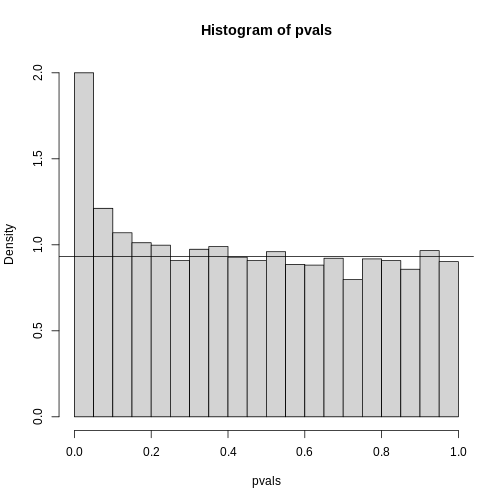
R
print(pi0) ##this is close to the try pi0=0.9
OUTPUT
[1] 0.9326667With this estimate in place we can, for example, alter the Benjamini and Hochberg procedures to select the \(k\) to be the largest value so that:
\[\hat{\pi}_0 p_{(i)} \leq \frac{i}{m}\alpha\]
However, instead of doing this, we compute a q-value for each test. If a feature resulted in a p-value of \(p\), the q-value is the estimated pFDR for a list of all the features with a p-value at least as small as \(p\).
In R, this can be computed with the qvalue function in
the qvalue package:
R
library(qvalue)
res <- qvalue(pvals)
qvals <- res$qvalues
plot(pvals, qvals)
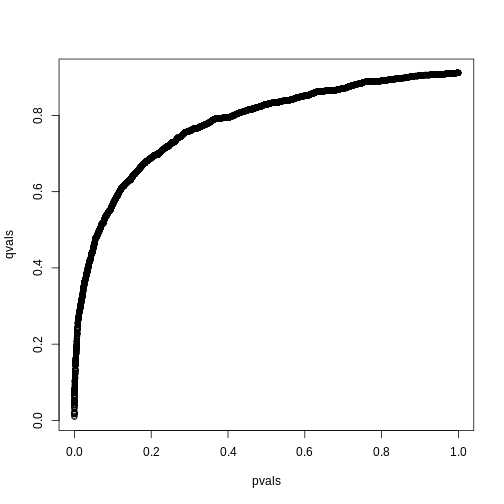
we also obtain the estimate of \(\hat{\pi}_0\):
R
res$pi0
OUTPUT
[1] 0.9117251This function uses a more sophisticated approach at estimating \(\pi_0\) than what is described above.
Exercises
In the following exercises, we will define error controlling procedures for experimental data. We will make a list of genes based on q-values. We will also assess your understanding of false positives rates and false negative rates by asking you to create a Monte Carlo simulation.
Exercise 1
Load the gene expression data:load("episodes/data/GSE5859Subset.rda")
We are interested in comparing gene expression between the two groups
defined in the sampleInfo table. Compute a p-value for each gene using
the function rowttests from the genefilter package.
library(genefilter)?rowttests
How many genes have p-values smaller than 0.05?
g <- sampleInfo$grouppvals <- rowttests(geneExpression, factor(g))$p.valuesum(pvals < 0.05)
Exercise 2: Apply the Bonferroni correction to achieve a FWER of 0.05. How many genes are called significant under this procedure?
m <- 8793sum(pvals < (0.05/m))
Exercise 3
The FDR is a property of a list of features, not each specific feature. The q-value relates FDR to individual features. To define the q-value, we order features we tested by p-value, then compute the FDRs for a list with the most significant, the two most significant, the three most significant, etc. The FDR of the list with the, say, m most significant tests is defined as the q-value of the m-th most significant feature. In other words, the q-value of a feature, is the FDR of the biggest list that includes that gene. In R, we can compute q-values using the p.adjust function with the FDR option. Read the help file for p.adjust and compute how many genes achieve a q-value < 0.05 for our gene expression dataset.
pvals_adjust <- p.adjust(pvals, method = 'fdr')sum(pvals_adjust < 0.05)
Exercise 4
Now use the qvalue function, in the Bioconductor qvalue package, to estimate q-values using the procedure described by Storey. How many genes have q-values below 0.05?
res <- qvalue(pvals)sum(res$qvalues < 0.05)
Exercise 5
Read the help file for qvalue and report the estimated proportion of genes for which the null hypothesis is true π0 = m0/m
res$pi0
Exercise 6
The number of genes passing the q-value < 0.05 threshold is larger
with the q-value function than the p.adjust difference. Why is this the
case? Make a plot of the ratio of these two estimates to help answer the
question.
A) One of the two procedures is flawed.
B) The two functions are estimating different things.
C) The qvalue function estimates the proportion of genes for which the
null hypothesis is true and provides a less conservative estimate.
D) The qvalue function estimates the proportion of genes for which the
null hypothesis is true and provides a more conservative estimate.
plot(pvals_adjust, res$qvalues, xlab = 'fdr', ylab = 'qval')abline(0,1)
The qvalue function estimates the proportion of genes for which the null
hypothesis is true and provides a less conservative estimate (choice
C).
Exercise 7
This exercise and the remaining ones are more advanced. Create a Monte Carlo Simulation in which you simulate measurements from 8,793 genes for 24 samples, 12 cases and 12 controls. Then for 100 genes create a difference of 1 between cases and controls. You can use the code provided below. Run this experiment 1,000 times with a Monte Carlo simulation. For each instance, compute p-values using a t-test and keep track of the number of false positives and false negatives. Compute the false positive rate and false negative rates if we use Bonferroni, q-values from p.adjust, and q-values from qvalue function. Set the seed to 1 for all three simulations. What is the false positive rate for Bonferroni? What are the false negative rates for Bonferroni?
n <- 24
m <- 8793
mat <- matrix(rnorm(n*m),m,n)
delta <- 1
positives <- 500
mat[1:positives,1:(n/2)] <- mat[1:positives,1:(n/2)]+delta g <- c(rep(0,12),rep(1,12))
m <- 8793
B <- 1000
m1 <- 500
N <- 12
m0 <- m-m1
nullHypothesis <- c(rep(TRUE,m0),rep(FALSE,m1))
delta <- 1
set.seed(1)
res <- replicate(B, {
controls <- matrix(rnorm(N*m),nrow = m, ncol = N)
treatment <- matrix(rnorm(N*m),nrow = m, ncol = N)
treatment[!nullHypothesis,] <-
treatment[!nullHypothesis,] + delta
dat <- cbind(controls, treatment)
pvals <- rowttests(dat, factor(g))$p.value
calls <- pvals < (0.05/m)
R <- sum(calls)
V <- sum(nullHypothesis & calls)
fp <- sum(nullHypothesis & calls)/m0 # false positive
fn <- sum(!nullHypothesis & !calls)/m1 # false negative
return(c(fp,fn))
})
res<-t(res)
head(res)
mean(res[,1]) # false positive rate
mean(res[,2]) # false negative rateExercise 8
What are the false positive rates for p.adjust?
What are the false negative rates for p.adjust?
g <- c(rep(0,12),rep(1,12))
m <- 8793
B <- 1000
m1 <- 500
N <- 12
m0 <- m-m1
nullHypothesis <- c(rep(TRUE,m0),rep(FALSE,m1))
delta <- 1

set.seed(1)
res <- replicate(B, {
  controls <- matrix(rnorm(N*m),nrow = m, ncol = N)
  treatment <- matrix(rnorm(N*m),nrow = m, ncol = N)
  treatment[!nullHypothesis,] <-
    treatment[!nullHypothesis,] + delta
  dat <- cbind(controls, treatment)
  pvals <- rowttests(dat, factor(g))$p.value
  pvals_adjust <- p.adjust(pvals, method = 'fdr')
  calls <- pvals_adjust < 0.05
  R <- sum(calls)
  V <- sum(nullHypothesis & calls)
  fp <- sum(nullHypothesis & calls)/m0 # false positive
  fn <- sum(!nullHypothesis & !calls)/m1 # false negative
  return(c(fp,fn))
})
res <- t(res)
head(res)
mean(res[,1]) # false positive rate
mean(res[,2]) # false negative rateExercise 9
What are the false positive rates for qvalues?
What are the false negative rates for qvalues?
g <- c(rep(0,12),rep(1,12))
m <- 8793
B <- 1000
m1 <- 500
N <- 12
m0 <- m-m1
nullHypothesis <- c(rep(TRUE,m0),rep(FALSE,m1))
delta <- 1

set.seed(1)
res <- replicate(B, {
  controls <- matrix(rnorm(N*m),nrow = m, ncol = N)
  treatment <- matrix(rnorm(N*m),nrow = m, ncol = N)
  treatment[!nullHypothesis,] <-
    treatment[!nullHypothesis,] + delta
  dat <- cbind(controls, treatment)
  pvals <- rowttests(dat, factor(g))$p.value
  qvals <- qvalue(pvals)$qvalue
  calls <- qvals < 0.05
  R <- sum(calls)
  V <- sum(nullHypothesis & calls)
  fp <- sum(nullHypothesis & calls)/m0 # false positive
  fn <- sum(!nullHypothesis & !calls)/m1 # false negative
  return(c(fp,fn))
})
res <- t(res)
head(res)
mean(res[,1]) # false positive rate
mean(res[,2]) # false negative rate - The Storey correction makes different assumptions that Benjamini-Hochberg. It does not set a priori alpha levels, but instead estimates the number of true null hypotheses from a given data set.
- The Storey correction is less computationally stable than Benjamini-Hochberg.