Procedures for Multiple Comparisons
Last updated on 2025-09-23 | Edit this page
Estimated time: 30 minutes
Overview
Questions
- Why are p-values not a useful quantity when dealing with high-dimensional data?
- What are error rates and how are they calculated?
Objectives
- Define multiple comparisons and the resulting problems.
- Explain terms associated with error rates.
- Explain the relationship between error rates and multiple comparisons.
Procedures
In the previous section we learned how p-values are no longer a useful quantity to interpret when dealing with high-dimensional data. This is because we are testing many features at the same time. We refer to this as the multiple comparison or multiple testing or multiplicity problem. The definition of a p-value does not provide a useful quantification here. Again, because when we test many hypotheses simultaneously, a list based simply on a small p-value cut-off of, say 0.01, can result in many false positives with high probability. Here we define terms that are more appropriate in the context of high-throughput data.
The most widely used approach to the multiplicity problem is to define a procedure and then estimate or control an informative error rate for this procedure. What we mean by control here is that we adapt the procedure to guarantee an error rate below a predefined value. The procedures are typically flexible through parameters or cutoffs that let us control specificity and sensitivity. An example of a procedure is:
- Compute a p-value for each gene.
- Call significant all genes with p-values smaller than \(\alpha\).
Note that changing the \(\alpha\) permits us to adjust specificity and sensitivity.
Next we define the error rates that we will try to estimate and control.
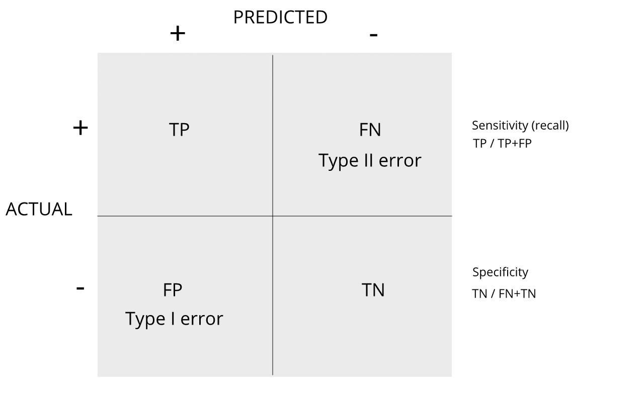
Review the matrix below to understand sensitivity, specificity, and error rates.
Discussion
Turn to a partner and explain the following:
1. Type I error
2. Type II error
3. sensitivity
4. specificity
When you are finished discussing, share with the group in the
collaborative document.
For more on this, see Classification evaluation by J. Lever, M. Krzywinski and N. Altman in Nature Methods 13, 603-604 (2016).
Exercises
With these exercises we hope to help you further grasp the concept that p-values are random variables and start laying the ground work for the development of procedures that control error rates. The calculations to compute error rates require us to understand the random behavior of p-values. We are going to ask you to perform some calculations related to introductory probability theory. One particular concept you need to understand is statistical independence. You also will need to know that the probability of two random e vents that are statistically independent occurring is P (A and B) = P (A)P (B). This is a consequence of the more general formula P (A and B) = P (A)P (B|A).
Exercise 1
Assume the null is true and denote the p-value you would get if you
ran a test as P. Define the function f (x) = Pr(P x) . What does f (x)
look like?
A) A uniform distribution.
B) The identity line.
C) A constant at 0.05.
D) P is not a random value.
Exercise 2
In the previous exercises, we saw how the probability of incorrectly rejecting the null for at least one of 20 experiments for which the null is true, is well over 5%. Now let’s consider a case in which we run thousands of tests, as we would do in a high throughput experiment. We previously learned that under the null, the probability of a p-value < p is p. If we run 8,793 independent tests, what it the probability of incorrectly rejecting at least one of the null hypothesis?
1 - 0.95^8793
Exercise 3
Suppose we need to run 8,793 statistical tests and we want to make the probability of a mistake very small, say 5%. Use the answer to Exercise 2 (Sidak’s procedure) to determine how small we have to change the cutoff, previously 0.05, to lower our probability of at least one mistake to be 5%.
m <- 87931 - 0.95^(1/m)
- We want our inferential analyses to maximize the percentage of true positives (sensitivity) and true negatives (specificity)
- p values are random variables, conducting multiple comparisons on high throughput data can produce a large number of false positives (Type 1 errors) simply by chance.
- There are procedures for improving sensitivity and specificity by controlling error rates below a predefined value.