Basic inference for high-throughput data
Last updated on 2025-09-23 | Edit this page
Estimated time: 60 minutes
Overview
Questions
- How are inferences from high-throughput data different from inferences from smaller samples?
- How is the interpretation of p-values affected by high-throughput data?
Objectives
- Demonstrate that p-values are random variables.
- Simulate p-values from multiple analyses of high-throughput data.
Inference in Practice
Suppose we were given high-throughput gene expression data that was measured for several individuals in two populations. We are asked to report which genes have different average expression levels in the two populations. If instead of thousands of genes, we were handed data from just one gene, we could simply apply the inference techniques that we have learned before. We could, for example, use a t-test or some other test. Here we review what changes when we consider high-throughput data.
p-values are random variables
An important concept to remember in order to understand the concepts presented in this chapter is that p-values are random variables. Let’s revisit random variables as addressed in this Statistical Inference for Biology episode. We have a dataset that we imagine contains the weights of all control female mice. We refer to this as the population, even though it is impossible to have data for all mice in population. For illustrative purposes we imagine having access to an entire population, though in practice we cannot.
To illustrate a random variable, sample 12 mice from the population three times and watch how the average changes.
R
population <- unlist(read.csv(file = "./data/femaleControlsPopulation.csv"))
R
control <- sample(population, 12)
mean(control)
OUTPUT
[1] 22.1925R
control <- sample(population, 12)
mean(control)
OUTPUT
[1] 24.75417R
control <- sample(population, 12)
mean(control)
OUTPUT
[1] 23.94333Notice that the mean is a random variable. To explore p-values as random variables, consider the example in which we define a p-value from a t-test with a large enough sample size to use the Central Limit Theorem (CLT) approximation. The CLT says that when the sample size is large, the average Ȳ of a random sample follows a normal distribution centered at the population average μY and with standard deviation equal to the population standard deviation σY, divided by the square root of the sample size N.Then our p-value is defined as the probability that a normally distributed random variable is larger, in absolute value, than the observed t-test, call it Z. Recall that a t-statistic is the ratio of the observed effect size and the standard error. Because it’s the ratio of two random variables, it too is a random variable. So for a two sided test the p-value is:
In R, we write:
R
2 * (1 - pnorm(abs(Z)))
Now because Z is a random variable and Φ is a deterministic function, p is also a random variable. We will create a Monte Carlo simulation showing how the values of p change.
We use replicate to repeatedly create p-values.
R
set.seed(1)
N <- 12
B <- 10000
pvals <- replicate(B, {
  control = sample(population, N)
  treatment = sample(population, N)
  t.test(treatment, control)$p.val
  })
hist(pvals)
As implied by the histogram, in this case the distribution of the p-value is uniformly distributed. In fact, we can show theoretically that when the null hypothesis is true, this is always the case. For the case in which we use the CLT, we have that the null hypothesis H0 implies that our test statistic Z follows a normal distribution with mean 0 and SD 1 thus:
 This implies that:
which is the definition of a uniform distribution.
Thousands of tests
In this data we have two groups denoted with 0 and 1:
R
load("data/GSE5859Subset.rda")
g <- sampleInfo$group
g
OUTPUT
[1] 1 1 1 1 1 1 1 1 1 1 1 1 0 0 0 0 0 0 0 0 0 0 0 0If we were interested in a particular gene, let’s arbitrarily pick the one on the 25th row, we would simply compute a t-test. To compute a p-value, we will use the t-distribution approximation and therefore we need the population data to be approximately normal. Recall that when the CLT does not apply (e.g. when sample sizes aren’t large enough), we can use the t-distribution.
We check our assumption that the population is normal with a qq-plot:
R
e <- geneExpression[25, ]
R
library(rafalib)
mypar(1,2)

qqnorm(e[g==1])
qqline(e[g==1])

qqnorm(e[g==0])
qqline(e[g==0])
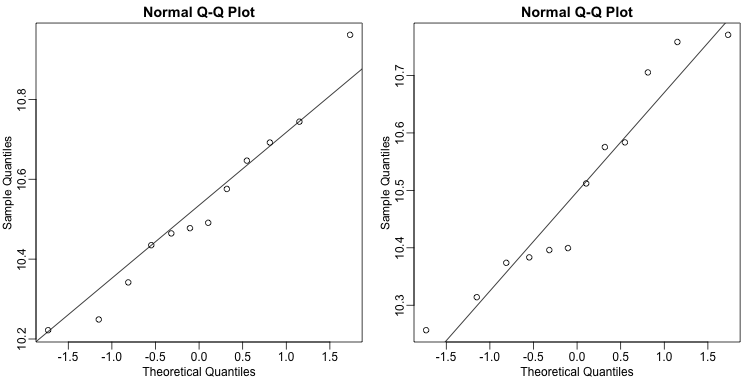
The qq-plots show that the data is well approximated by the normal approximation. The t-test does not find this gene to be statistically significant:
R
t.test(e[g==1], e[g==0])$p.value
OUTPUT
[1] 0.779303To answer the question for each gene, we simply repeat the above for
each gene. Here we will define our own function and use
apply:
R
myttest <- function(x)
  t.test(x[g==1],
         x[g==0],
         var.equal=TRUE)$p.value
pvals <- apply(geneExpression, 1, myttest)
We can now see which genes have p-values less than, say, 0.05. For example, right away we see that…
R
sum(pvals < 0.05)
OUTPUT
[1] 1383… genes had p-values less than 0.05.
However, as we will describe in more detail below, we have to be careful in interpreting this result because we have performed over 8,000 tests. If we performed the same procedure on random data, for which the null hypothesis is true for all features, we obtain the following results:
R
set.seed(1)
m <- nrow(geneExpression)
n <- ncol(geneExpression)
randomData <- matrix(rnorm(n * m), m, n)
nullpvals <- apply(randomData, 1, myttest)
sum(nullpvals < 0.05)
OUTPUT
[1] 419Discussion
Turn to a partner and explain what you did and found in the previous two analyses. What do you think the results mean? Then, share your responses with the group through the collaborative document.
As we will explain later in the chapter, this is to be expected: 419 is roughly 0.05 * 8192 and we will describe the theory that tells us why this prediction works.
Faster t-test implementation
Before we continue, we should point out that the above implementation is very inefficient. There are several faster implementations that perform t-test for high-throughput data. We make use of a function that is not available from CRAN, but rather from the Bioconductor project. Now we can show that this function is much faster than our code above and produce practically the same answer:
R
library(genefilter)
results <- rowttests(geneExpression, factor(g))
max(abs(pvals - results$p))
OUTPUT
[1] 6.528111e-14Exercises
These exercises will help clarify that p-values are random variables
and some of the properties of these p-values. Note that just like the
sample average is a random variable because it is based on a random
sample, the p-values are based on random variables (sample mean and
sample standard deviation for example) and thus it is also a random
variable.
To see this, let’s see how p-values change when we take different
samples.
R
set.seed(1)
pvals <- replicate(1000, { # recreate p-values as from above
  control = sample(population, 12)
  treatment = sample(population, 12)
  t.test(treatment,control)$p.val
  }
  )
head(pvals)
OUTPUT
[1] 0.3191557945 0.2683723148 0.0003358878 0.0312671917 0.1410320545
[6] 0.9478677657
R
hist(pvals)
Exercise 1: What proportion of the p-values is below 0.05?
sum(pvals < 0.05)/length(pvals)
50 of the p-values are less than 0.05 of a total
1000 p-values
Exercise 2: What proportion of the p-values is below 0.01?
sum(pvals < 0.01)/length(pvals)
11 of the p-values are less than 0.01 of a total
1000 p-values
Exercise 3
Assume you are testing the effectiveness of 20 diets on mice weight. For each of the 20 diets, you run an experiment with 10 control mice and 10 treated mice. Assume the null hypothesis, that the diet has no effect, is true for all 20 diets and that mice weights follow a normal distribution, with mean 30 grams and a standard deviation of 2 grams. Run a Monte Carlo simulation for one of these studies:
cases = rnorm(10, 30, 2)
controls = rnorm(10, 30, 2)
t.test(cases, controls)
Now run a Monte Carlo simulation imitating the results for the experiment for all 20 diets. If you set the seed at 100, set.seed(100), how many of p-values are below 0.05?
set.seed(100)n <- 20null <- vector("numeric", n)for (i in 1:n) {cases = rnorm(10, 30, 2)controls = rnorm(10, 30, 2)null[i] <- t.test(cases, controls)$p.val}sum(null < 0.05)
Exercise 4
Now create a simulation to learn about the distribution of the number of p-values that are less than 0.05. In question 3, we ran the 20 diet experiment once. Now we will run the experiment 1,000 times and each time save the number of p-values that are less than 0.05. Set the seed at 100, set.seed(100), run the code from Question 3 1,000 times, and save the number of times the p-value is less than 0.05 for each of the 1,000 instances. What is the average of these numbers? This is the expected number of tests (out of the 20 we run) that we will reject when the null is true.
set.seed(100)res <- replicate(1000, {randomData <- matrix(rnorm(20*20,30,2),20,20)pvals <- rowttests(randomData, factor(g))$p.valuereturn(sum(pvals<0.05)) # total number of false
positives per replication})mean(res)
Exercise 5
What this says is that on average, we expect some p-value to be 0.05 even when the null is true for all diets. Use the same simulation data and report for what percent of the 1,000 replications did we make more than 0 false positives?
mean(res 0)
- P-values are random variables.
- Very small p-values can occur by random chance when analyzing high-throughput data.