Calculating Genotype Probabilities
Overview
Teaching: 30 min
Exercises: 30 minQuestions
How do I calculate QTL at positions between genotyped markers?
How do I calculate QTL genotype probabilities?
How do I calculate allele probabilities?
How can I speed up calculations if I have a large data set?
Objectives
To explain why the first step in QTL analysis is to calculate genotype probabilities.
To insert pseudomarkers between genotyped markers.
To calculate genotype probabilities.
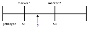
The first task in QTL analysis is to calculate conditional genotype probabilities, given the observed marker data, at each putative QTL position. For example, the first step would be to determine the probabilities for genotypes SS and SB at the locus indicated below.
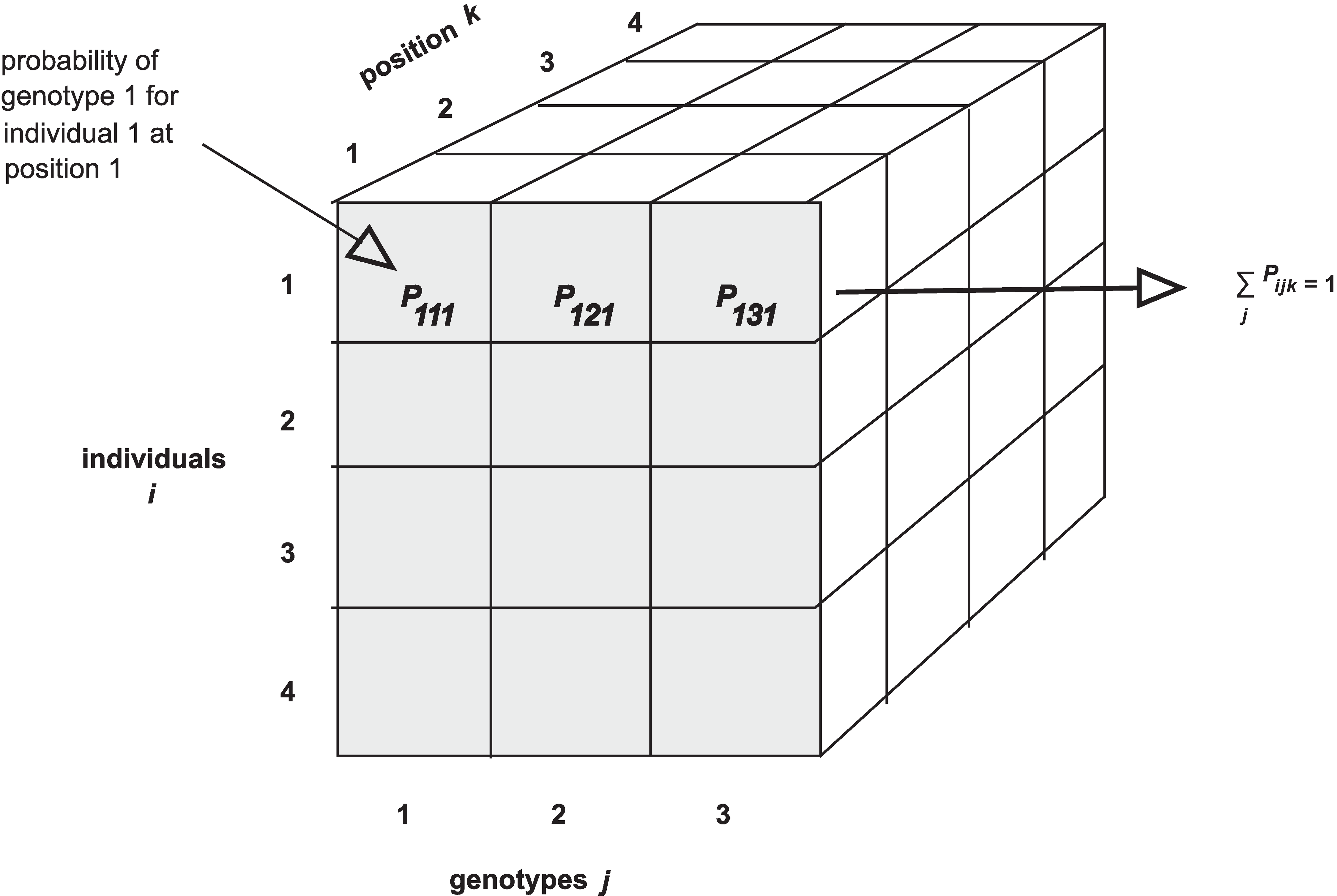
The calc_genoprob() function calculates QTL genotype probabilities, conditional on the available marker data. These are needed for most of the QTL mapping functions. The result is returned as a list of three-dimensional arrays (one per chromosome). Each 3d array of probabilities is arranged as individuals × genotypes × positions.
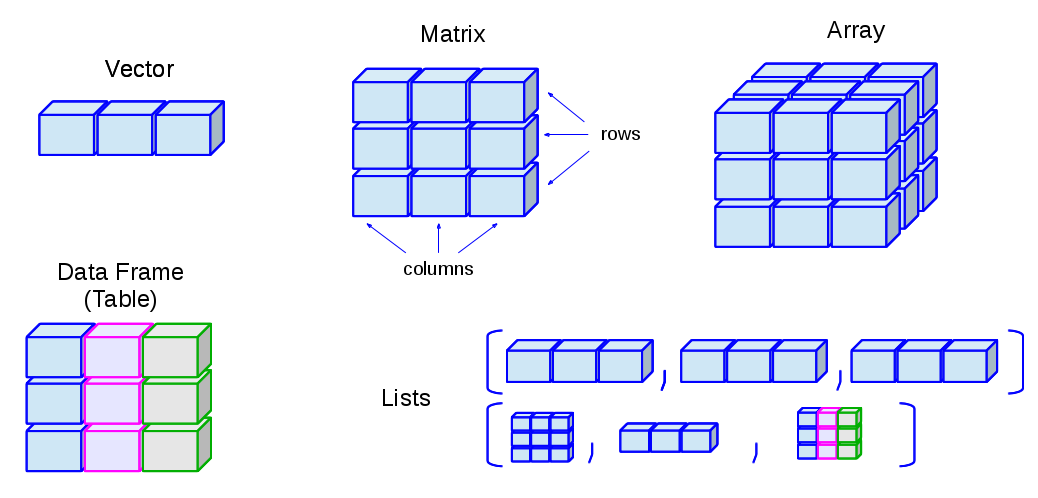
See this page for a graphical review of data structures in R.
To find QTL at positions between markers (so called “pseudomarkers”), first insert pseudomarkers into the genetic map with the function insert_pseudomarkers().
We’ll use the iron dataset from Grant et al. (2006) Hepatology 44:174-185 (an intercross) as an example. In this study spleen and liver iron levels were measured in an F2 cross between mouse strains C57BL/6J and SWR. C57BL/6J mice exhibit low levels of non-heme iron, while SWR mice exhibit high levels. Iron levels between spleen and liver in the F2s were poorly correlated, indicating tissue-specific regulation. Significant QTL were found on chromosomes 2 and 16 for liver, and on chromosomes 8 and 9 in spleen. Candidate genes included transferrin near the chromosome 9 peak, and β2-microglobulin near the chromosome 2 peak.
We first load the data using the function system.file, which finds files located in packages. The iron data are built into the qtl2 package, so we can use the system.file() function to load them directly from the package.
library(qtl2)
iron <- read_cross2(file = system.file("extdata", "iron.zip", package="qtl2") )
To load your own data from your machine, you would use the file path to your data files. For example, if the file path to your data files is /Users/myUserName/qtlProject/data, the command to load your data would look like this:
myQTLdata <- read_cross2(file = "/Users/myUserName/qtlProject/data/myqtldata.yaml" )
The YAML file contains all control information for your data, including names of data files, cross type, column specifications for sex and cross information, and more. This can also be in JSON format. Alternatively, all data files can be zipped together for loading.
myQTLdata <- read_cross2(file = "/Users/myUserName/qtlProject/data/myqtldata.zip" )
Back to the iron data. Now look at a summary of the cross data and the names of each variable within the data.
summary(iron)
Object of class cross2 (crosstype "f2")

Total individuals            284
No. genotyped individuals    284
No. phenotyped individuals   284
No. with both geno & pheno   284

No. phenotypes                 2
No. covariates                 2
No. phenotype covariates       1

No. chromosomes               20
Total markers                 66

No. markers by chr:
 1  2  3  4  5  6  7  8  9 10 11 12 13 14 15 16 17 18 19  X
 3  5  2  2  2  2  7  8  5  2  7  2  2  2  2  5  2  2  2  2
names(iron)
 [1] "crosstype"  "geno"       "gmap"       "pmap"       "pheno"
 [6] "covar"      "phenocovar" "is_x_chr"   "is_female"  "cross_info"
[11] "alleles"
Have a look at the markers listed in the genetic map, gmap. Markers are listed by chromosome and described by cM position. View only the markers on the first several chromosomes.
head(iron$gmap)
$`1`
D1Mit18 D1Mit80 D1Mit17
   27.3    51.4   110.4

$`2`
D2Mit379  D2Mit75  D2Mit17 D2Mit304  D2Mit48
    38.3     48.1     56.8     58.0     73.2

$`3`
D3Mit22 D3Mit18
   25.1    54.6

$`4`
  D4Mit2 D4Mit352
    10.9     53.6

$`5`
D5Mit11 D5Mit30
   17.5    62.3

$`6`
D6Mit104  D6Mit15
    41.5     66.7
We then use insert_pseudomarkers() to insert pseudomarkers into the
genetic map, which we grab from the iron object as iron$gmap:
map <- insert_pseudomarkers(map=iron$gmap, step=1)
Pseudomarkers are inserted at regular intervals, and genotype probabilities will be calculated at each of these intervals. Now have a look at the new object called map. View only the first two chromosomes.
head(map, n=2)
$`1`
  D1Mit18  c1.loc28  c1.loc29  c1.loc30  c1.loc31  c1.loc32  c1.loc33  c1.loc34
     27.3      28.3      29.3      30.3      31.3      32.3      33.3      34.3
 c1.loc35  c1.loc36  c1.loc37  c1.loc38  c1.loc39  c1.loc40  c1.loc41  c1.loc42
     35.3      36.3      37.3      38.3      39.3      40.3      41.3      42.3
 c1.loc43  c1.loc44  c1.loc45  c1.loc46  c1.loc47  c1.loc48  c1.loc49  c1.loc50
     43.3      44.3      45.3      46.3      47.3      48.3      49.3      50.3
 c1.loc51   D1Mit80  c1.loc52  c1.loc53  c1.loc54  c1.loc55  c1.loc56  c1.loc57
     51.3      51.4      52.3      53.3      54.3      55.3      56.3      57.3
 c1.loc58  c1.loc59  c1.loc60  c1.loc61  c1.loc62  c1.loc63  c1.loc64  c1.loc65
     58.3      59.3      60.3      61.3      62.3      63.3      64.3      65.3
 c1.loc66  c1.loc67  c1.loc68  c1.loc69  c1.loc70  c1.loc71  c1.loc72  c1.loc73
     66.3      67.3      68.3      69.3      70.3      71.3      72.3      73.3
 c1.loc74  c1.loc75  c1.loc76  c1.loc77  c1.loc78  c1.loc79  c1.loc80  c1.loc81
     74.3      75.3      76.3      77.3      78.3      79.3      80.3      81.3
 c1.loc82  c1.loc83  c1.loc84  c1.loc85  c1.loc86  c1.loc87  c1.loc88  c1.loc89
     82.3      83.3      84.3      85.3      86.3      87.3      88.3      89.3
 c1.loc90  c1.loc91  c1.loc92  c1.loc93  c1.loc94  c1.loc95  c1.loc96  c1.loc97
     90.3      91.3      92.3      93.3      94.3      95.3      96.3      97.3
 c1.loc98  c1.loc99 c1.loc100 c1.loc101 c1.loc102 c1.loc103 c1.loc104 c1.loc105
     98.3      99.3     100.3     101.3     102.3     103.3     104.3     105.3
c1.loc106 c1.loc107 c1.loc108 c1.loc109 c1.loc110   D1Mit17
    106.3     107.3     108.3     109.3     110.3     110.4

$`2`
D2Mit379 c2.loc39 c2.loc40 c2.loc41 c2.loc42 c2.loc43 c2.loc44 c2.loc45
    38.3     39.3     40.3     41.3     42.3     43.3     44.3     45.3
c2.loc46 c2.loc47  D2Mit75 c2.loc48 c2.loc49 c2.loc50 c2.loc51 c2.loc52
    46.3     47.3     48.1     48.3     49.3     50.3     51.3     52.3
c2.loc53 c2.loc54 c2.loc55 c2.loc56  D2Mit17 c2.loc57 D2Mit304 c2.loc58
    53.3     54.3     55.3     56.3     56.8     57.3     58.0     58.3
c2.loc59 c2.loc60 c2.loc61 c2.loc62 c2.loc63 c2.loc64 c2.loc65 c2.loc66
    59.3     60.3     61.3     62.3     63.3     64.3     65.3     66.3
c2.loc67 c2.loc68 c2.loc69 c2.loc70 c2.loc71 c2.loc72  D2Mit48
    67.3     68.3     69.3     70.3     71.3     72.3     73.2
Notice that pseudomarkers are now spaced at 1 cM intervals from genotyped markers. The argument step=1 generated pseudomarkers at these intervals.
Next we use calc_genoprob() to calculate the QTL genotype probabilities.
pr <- calc_genoprob(cross=iron, map=map, error_prob=0.002)
The argument error_prob supplies an assumed genotyping error probability of 0.002. If a value for error_prob is not supplied, the default probability is 0.0001.
Recall that the result of calc_genoprob, pr, is a list of three-dimensional arrays (one per chromosome).
names(pr)
 [1] "1"  "2"  "3"  "4"  "5"  "6"  "7"  "8"  "9"  "10" "11" "12" "13" "14" "15"
[16] "16" "17" "18" "19" "X"
Each three-dimensional array of probabilities is arranged as individuals × genotypes × positions. Have a look at the names of each of the three dimensions for chromosome 19.
dimnames(pr$`19`)
[[1]]
  [1] "1"   "2"   "3"   "4"   "5"   "6"   "7"   "8"   "9"   "10"  "11"  "12"
 [13] "13"  "14"  "15"  "16"  "17"  "18"  "19"  "20"  "21"  "22"  "23"  "24"
 [25] "25"  "26"  "27"  "28"  "29"  "30"  "31"  "32"  "33"  "34"  "35"  "36"
 [37] "37"  "38"  "39"  "40"  "41"  "42"  "43"  "44"  "45"  "46"  "47"  "48"
 [49] "49"  "50"  "51"  "52"  "53"  "54"  "55"  "56"  "57"  "58"  "59"  "60"
 [61] "61"  "62"  "63"  "64"  "65"  "66"  "67"  "68"  "69"  "70"  "71"  "72"
 [73] "73"  "74"  "75"  "76"  "77"  "78"  "79"  "80"  "81"  "82"  "83"  "84"
 [85] "85"  "86"  "87"  "88"  "89"  "90"  "91"  "92"  "93"  "94"  "95"  "96"
 [97] "97"  "98"  "99"  "100" "101" "102" "103" "104" "105" "106" "107" "108"
[109] "109" "110" "111" "112" "113" "114" "115" "116" "117" "118" "119" "120"
[121] "121" "122" "123" "124" "125" "126" "127" "128" "129" "130" "131" "132"
[133] "133" "134" "135" "136" "137" "138" "139" "140" "141" "142" "143" "144"
[145] "145" "146" "147" "148" "149" "150" "151" "152" "153" "154" "155" "156"
[157] "157" "158" "159" "160" "161" "162" "163" "164" "165" "166" "167" "168"
[169] "169" "170" "171" "172" "173" "174" "175" "176" "177" "178" "179" "180"
[181] "181" "182" "183" "184" "185" "186" "187" "188" "189" "190" "191" "192"
[193] "193" "194" "195" "196" "197" "198" "199" "200" "201" "202" "203" "204"
[205] "205" "206" "207" "208" "209" "210" "211" "212" "213" "214" "215" "216"
[217] "217" "218" "219" "220" "221" "222" "223" "224" "225" "226" "227" "228"
[229] "229" "230" "231" "232" "233" "234" "235" "236" "237" "238" "239" "240"
[241] "241" "242" "243" "244" "245" "246" "247" "248" "249" "250" "251" "252"
[253] "253" "254" "255" "256" "257" "258" "259" "260" "261" "262" "263" "264"
[265] "265" "266" "267" "268" "269" "270" "271" "272" "273" "274" "275" "276"
[277] "277" "278" "279" "280" "281" "282" "283" "284"

[[2]]
[1] "SS" "SB" "BB"

[[3]]
 [1] "D19Mit68"  "c19.loc4"  "c19.loc5"  "c19.loc6"  "c19.loc7"  "c19.loc8"
 [7] "c19.loc9"  "c19.loc10" "c19.loc11" "c19.loc12" "c19.loc13" "c19.loc14"
[13] "c19.loc15" "c19.loc16" "c19.loc17" "c19.loc18" "c19.loc19" "c19.loc20"
[19] "c19.loc21" "c19.loc22" "c19.loc23" "c19.loc24" "c19.loc25" "c19.loc26"
[25] "c19.loc27" "c19.loc28" "c19.loc29" "c19.loc30" "c19.loc31" "c19.loc32"
[31] "c19.loc33" "c19.loc34" "c19.loc35" "c19.loc36" "c19.loc37" "D19Mit37"
View the first three rows of genotype probabilities for the first genotyped marker on chromosome 19, and the two adjacent pseudomarkers located at 1 cM intervals away. Compare the probabilities for each pseudomarker genotype with those of the genotyped marker.
(pr$`19`)[1:3,,"D19Mit68"] # genotyped marker
            SS          SB           BB
1 0.0009976995 0.003298162 0.9957041387
2 0.2500000000 0.500000000 0.2500000000
3 0.0003029243 0.999394151 0.0003029243
(pr$`19`)[1:3,,"c19.loc4"] # pseudomarker 1 cM away
           SS         SB          BB
1 0.001080613 0.03581825 0.963101136
2 0.250000000 0.50000000 0.250000000
3 0.006141104 0.98771779 0.006141104
(pr$`19`)[1:3,,"c19.loc5"] # the next pseudomarker
           SS         SB         BB
1 0.001342511 0.06759555 0.93106194
2 0.250000000 0.50000000 0.25000000
3 0.011589058 0.97682188 0.01158906
We can also view the genotype probabilities using plot_genoprob. The arguments to this function specify:
- pr: the genotype probabilities,
- map: the marker map,
- ind: the index of the individual to plot,
- chr: the index of the chromosome to plot.
plot_genoprob(pr, map, ind = 1, chr = 19)

The coordinates along chromosome 19 are shown on the horizontal axis and the three genotypes are shown on the vertical axis. Higher genotype probabilities are plotted in darker shades. This mouse has a BB genotype on the proximal end of the chromosome and transitions to SB toward the distal end.
Challenge 1
Find a partner and explain why calculating genotype probabilities is the first step in QTL analysis. Why do you need to insert pseudomarkers first? Listen to your partner’s explanation, then write your responses in the collaborative document.
Solution to Challenge 1
Challenge 2
1). Load a second dataset from Arabidopsis recombinant inbred lines (Moore et al, Genetics, 2013) in a study of plant root response to gravity (gravitropism).
grav <- read_cross2(file = system.file('extdata', 'grav2.zip', package = 'qtl2'))
2). How many individuals were in the study? How many phenotypes? How many chromosomes?
3). Insert pseudomarkers at 1cM intervals and save the results to an object calledgravmap. Have a look at the first chromosome.
4). Calculate genotype probabilities and save the results to an object calledgravpr. View the genotypes for the first three markers and pseudomarkers on chromosome 1 for the first five individuals.Solution to Challenge 2
1).
grav <- read_cross2(file = system.file('extdata', 'grav2.zip', package = 'qtl2'))
2).summary(grav)
3).gravmap <- insert_pseudomarkers(map = grav$gmap, step = 1)
followed byhead(gravmap, n=1)
4).gravpr <- calc_genoprob(cross = grav, map = gravmap)followed by
(gravpr$1)[1:5,,"PVV4"],(gravpr$1)[1:5,,"c1.loc1"], and
(gravpr$1)[1:5,,"c1.loc2"]
Challenge 3
Calculate genotype probabilities for a different data set from the qtl2 data repository, this one from a study of obesity and diabetes in a C57BL/6 (B6) × BTBR intercross.
1). Create a new script in RStudio with File -> New File -> R Script.
2) Download the B6 x BTBR zip file from the qtl2 data repository into an object calledb6btbrby running this code:
b6btbr <- read_cross2(file = "https://raw.githubusercontent.com/rqtl/qtl2data/master/B6BTBR/b6btbr.zip")
3). View a summary of theb6btbrdata. How many individuals? phenotypes? chromosomes? markers?
4). View the genetic map for theb6btbrdata.
5). Insert pseudomarkers at 2 cM intervals. Assign the results to an object calledb6btbrmap.
6). Calculate genotype probabilities assuming a genotyping error probability of 0.001. Assign the results to an object calledb6btbrpr.
7). View the first several rows of genotype probabilities for any marker on chromosome 18.Solution to Challenge 3
1). Create a new script in RStudio with File -> New File -> R Script.
2).b6btbr <- read_cross2(file = "https://raw.githubusercontent.com/rqtl/qtl2data/master/B6BTBR/b6btbr.zip
3).summary(b6btbr)shows 544 individuals, 3 phenotypes, 20 chromosomes, 2057 markers.
4).b6btbr$gmap
5).b6btbrmap <- insert_pseudomarkers(map=b6btbr$gmap, step=2)
6).b6btbrpr <- calc_genoprob(cross=b6btbr, map=b6btbrmap, error_prob=0.001)
7).dimnames((b6btbrpr$18))shows all marker names for chromosome 18.head((b6btbrpr$18)[,,"c18.loc48"])gives genotype probabilities for an example pseudomarker, whilehead((b6btbrpr$18)[,,"rs6338896"])gives genotype probabilities for a genotyped marker.
Parallel calculations (optional) To speed up the calculations with large datasets on a multi-core machine, you can use the argument cores. With cores=0, the number of available cores will be detected via parallel::detectCores(). Otherwise, specify the number of cores as a positive integer.
pr <- calc_genoprob(cross=iron, map=map, error_prob=0.002, cores=4)
Allele probabilities (optional) The genome scan functions use genotype probabilities as well as a matrix of phenotypes. If you wished to perform a genome scan via an additive allele model, you would first convert the genotype probabilities to allele probabilities, using the function genoprob_to_alleleprob().
apr <- genoprob_to_alleleprob(probs=pr)
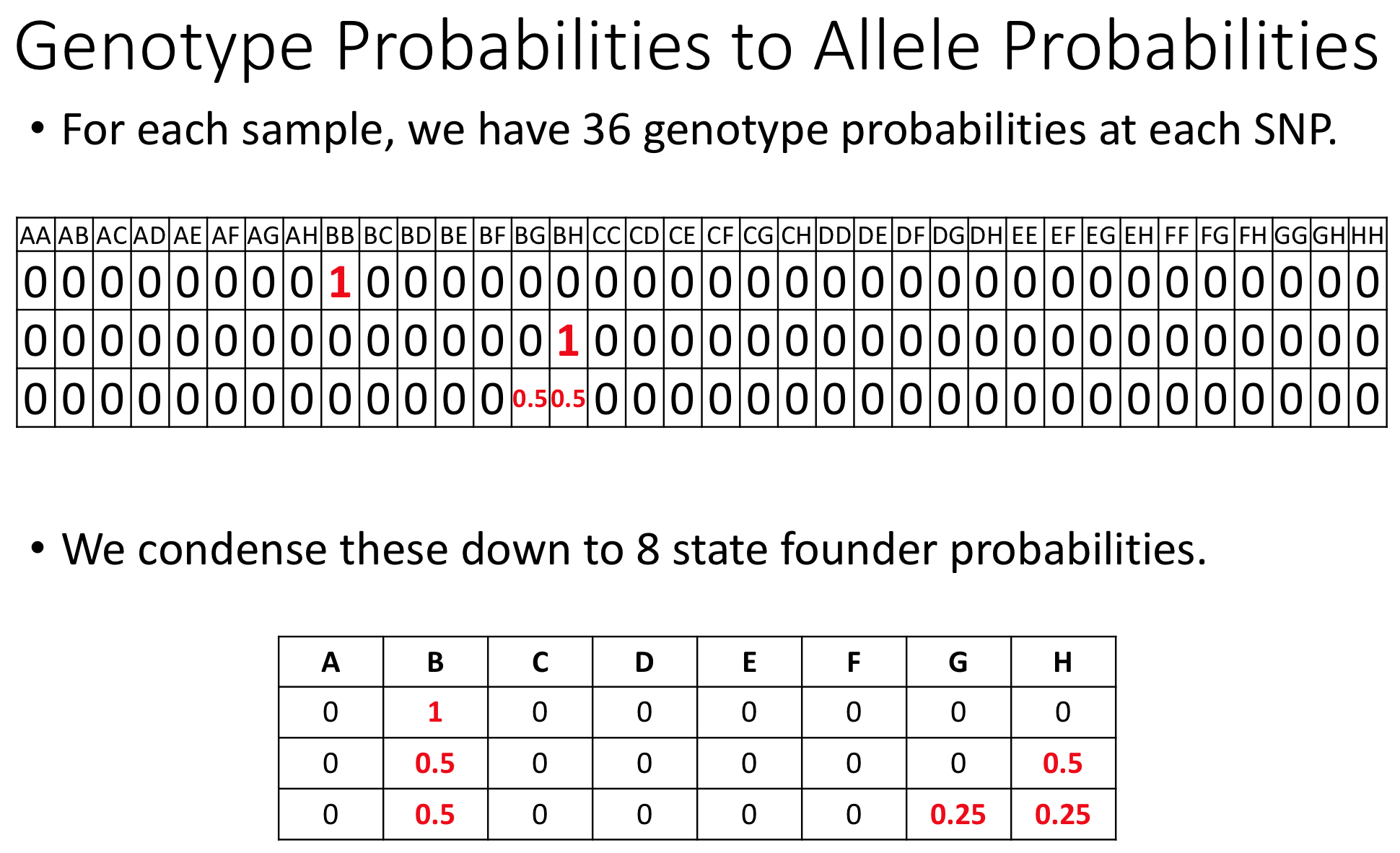
The figure below shows genotype and allele probabilities for 3 samples. In the Diversity Outbred, there are 36 possible genotype states (AA, AB, AC, …, BB, BC, BD, …, CC, CD, CE, …, DD, DE, DF, …, EE,…) or 8 + 7 + 6 + 5 + 4 + 3 + 2 + 1. The first SNP below has genotype BB. In the table describing alleles (8 state founder probabilities), the probability that this SNP has a B allele is 1. The 2nd SNP has genotype BH, so the allele table shows a probability of 0.5 for B and 0.5 for H. The third SNP is either BG or BH, and has a probability of 0.5 for each of these genotypes. The allele table shows a probability of 0.5 for allele B, and 0.25 for both G and H.
Key Points
The first step in QTL analysis is to calculate genotype probabilities.
Insert pseudomarkers to calculate QTL at positions between genotyped markers.
Calculate genotype probabilities between genotyped markers with calc_genoprob().