SNP association mapping

Overview

Teaching: 30 min
Exercises: 30 min

Questions

How do I identify SNPs in a QTL?

Objectives

Perform a basic QTL analysis.

Identify QTL with a genome scan.

Find SNPs within a QTL.

Convert founder genotypes to a strain distribution pattern (SDP).

Infer SNP genotypes for Diversity Outbred mice.

Perform SNP association analysis

For multi-parent crosses, it can be useful to collapse the genotype or allele probabilities according to the founder genotypes of the various SNPs in the region of a QTL.

QTL analysis in Diversity Outbred mice

To illustrate this sort of SNP association analysis, we’ll consider some Diversity Outbred mouse data. The Diversity Outcross (DO) mice are an advanced intercross population derived from the same eight founder strains as the Collaborative Cross (CC). See Svenson et al. (2012) and Gatti et al. (2014).

We’ll consider a subset of the data from Recla et al. (2014), available as part of the qtl2data github repository. (The full data are in DO_Recla; the directory DOex contains a reduced set, with just three chromosomes, one phenotype (OF_immobile_pct, percent immobile in the open field test), and a reduced set of markers.

You can download the data from a single zip file, as follows:

DOex <- read_cross2(file = "https://raw.githubusercontent.com/rqtl/qtl2data/master/DOex/DOex.zip")

Let’s quickly whip through a basic analysis.

We first calculate genotype probabilities and convert them to allele probabilities. We’ll just use marker locations and not insert any pseudomarkers.

pr <- calc_genoprob(DOex, error_prob=0.002)
apr <- genoprob_to_alleleprob(pr)

We calculate kinship matrices (using the “LOCO” method, though with the caveat that here we are only considering genotypes on three chromosomes).

k <- calc_kinship(apr, "loco")

We create a numeric covariate for sex; be sure to include the individual IDs as names.

sex <- (DOex$covar$Sex == "male")*1
names(sex) <- rownames(DOex$covar)

Note that you can create the vector and assign the names in one step using the basic R function setNames().

sex <- setNames( (DOex$covar$Sex == "male")*1, rownames(DOex$covar) )

We perform a genome scan with a linear mixed model (adjusting for a residual polygenic effect), with sex as an additive covariate.

out <- scan1(apr, DOex$pheno, k, sex)

Here’s a plot of the results.

par(mar=c(4.1, 4.1, 0.6, 0.6))
plot(out, DOex$gmap)

plot of chunk plot_DOex_scan

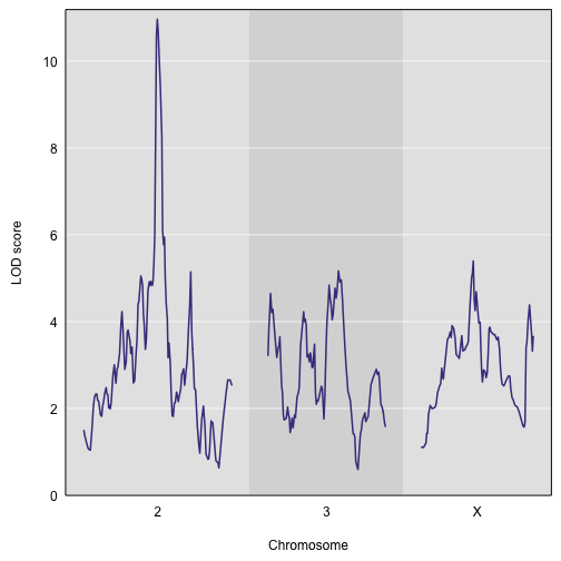
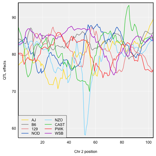
There’s a strong peak on chromosome 2. Let’s look at the QTL effects. We estimate them with scan1coef(). We need to subset the allele probabilities and the list of kinship matrices.

coef_c2 <- scan1coef(apr[,"2"], DOex$pheno, k[["2"]], sex)

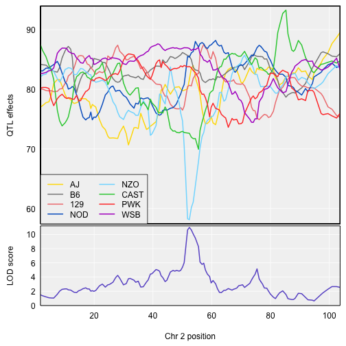
For the DO, with 8 QTL alleles, we can use the function plot_coefCC in the R/qtl2plot package, which plots the 8 allele effects in the “official” Collaborative Cross (CC) colors. (Well, actually slightly modified colors, because I think the official colors are kind of ugly.) The strong locus seems to be mostly due to the NZO allele. Note that CCcolors is a vector of colors included in the qtl2plot package; there’s also a CCorigcolors object with the official colors.

par(mar=c(4.1, 4.1, 0.6, 0.6))
plot_coefCC(coef_c2, DOex$gmap["2"], bgcolor="gray95", legend="bottomleft")

plot of chunk plot_DOex_effects

If you provide plot_coefCC() with the genome scan output, it will display the LOD curve below the coefficient estimates.

par(mar=c(4.1, 4.1, 0.6, 0.6))
plot_coefCC(coef_c2, DOex$gmap["2"], scan1_output=out, bgcolor="gray95", legend="bottomleft")

plot of chunk plot_DOex_lod_curve

Connecting to SNP and gene databases

To perform SNP association analysis in the region of a QTL, we’ll need to grab data on all of the SNPs in the region, including their genotypes in the eight founder strains for the CC and DO populations. As a related task, we’ll also want to identify the genes in the region.

We want R/qtl2 to permit different ways of storing this information. For the CC and DO populations, we’ve prepared SQLite database files for the variants in the CC founders and for the MGI mouse gene annotations. But others might wish to use a different kind of database, or may wish to query an online database.

We provide a template for how to use R/qtl2 to connect to SNP and gene databases, with the functions create_variant_query_func() and create_gene_query_func(). Each returns a function for querying variant and gene databases, respectively. The query functions that are returned take just three arguments (chr, start, end end), and themselves return a data frame of variants on the one hand and genes on the other.

During setup you would have downloaded the SQLite databases from Figshare and placed these in your data directory:

SQLite database of variants in Collaborative Cross founder mouse strains (v3): SNP, indel, and structural variants in the Collaborative Cross founders (3.87 GB)
SQLite database with mouse gene annotations from Mouse Genome Informatics (v6): full set of mouse gene annotations from build 38 mm10 (529.89 MB)
SQLite database with MGI mouse gene annotations from Mouse Genome Informatics (v7): like the previous, but including only non-duplicate gene records sourced from MGI (11.16 MB)

To create a function for querying the CC variants, call create_variant_query_func() with the path to the cc_variants.sqlite file:

query_variants <- create_variant_query_func("../data/cc_variants.sqlite")

To grab the variants in the interval 97-98 Mbp on chromosome 2, you’d then do the following:

variants_2_97.5 <- query_variants(2, 97, 98)

Similarly, to create a function for querying the MGI mouse gene annotations, you call create_gene_query_func() with the path to the mouse_genes_mgi.sqlite file:

query_genes <- create_gene_query_func("../data/mouse_genes_mgi.sqlite")

To grab the genes overlapping the interval 97-98 Mbp on chromosome 2, you’d then do the following:

genes_2_97.5 <- query_genes(2, 97, 98)

The way we’ve set this up is a bit complicated, but it allows greatest flexibility on the part of the user. And for our own work, we like to have a local SQLite database, for rapid queries of SNPs and genes.

SNP associations

Okay, now finally we get to the SNP associations. We have a large peak on chromosome 2, and we want to look at individual SNPs in the region of the locus.

Well, actually, we first need to find the location of the inferred QTL. The peak LOD score on chromosome 2 occurs at 52.4 cM. But to find nearby SNPs, we really want to know the Mbp position. The calculations were only performed at the marker positions, and so we can use max(), giving both the scan1() output and the physical map, and then pull out the position from the results.

peak_Mbp <- max(out, DOex$pmap)$pos

The marker is at 97.5 Mbp. We’ll focus on a 2 Mbp interval centered at 97.5 Mbp.

We can pull out the variants in the 2 Mbp interval centered at 97.5 on chr 2 using the query function we defined above:

variants <- query_variants(2, peak_Mbp - 1, peak_Mbp + 1)

There are 27355 variants in the interval, including 27108 SNPs, 127 indels, and 120 structural variants. We’re treating all of them as biallelic markers (all but the major allele in the eight founder strains binned into a single allele). In the following, we’re going to just say “SNP” rather than “variant”, even though the variants include indels and structural variants.

After identifying the variants in the interval of interest, we use our genotype probabilities and the founder SNP genotypes to infer the SNP genotypes for the DO mice. That is, at each SNP, we want to collapse the eight founder allele probabilities to two SNP allele probabilities, using the SNP genotypes of the founders.

We do this assuming that the genotype probabilities were calculated sufficiently densely that they can be assumed to be constant in intervals. With this assumption, we then:

Find the interval for each SNP.
Reduce the SNPs to a “distinct” set: if two SNPs have the same strain distribution pattern (SDP; the pattern of alleles in the eight founders) and are in the same interval, by our assumption their allele probabilities will be the same.
Take the average of the allele probabilities at the two endpoints of each interval.
Collapse the 8 allele probabilities to two according to each observed SDP in the interval.
We further create a look-up table relating the full set of SNPs to the reduced set (one of each observed SDP in each interval).

All of these steps are combined into a single function scan1snps(), which takes the genotype probabilities, a physical map of those locations, the phenotype, the kinship matrix, covariates, the query function for grabbing the SNPs in a given interval, and the chromosome, start, and end positions for the interval. (If insert_pseudomarkers() was used to insert pseudomarkers, you will need to use interp_map() to get interpolated Mbp positions for the pseudomarkers.)

out_snps <- scan1snps(pr, DOex$pmap, DOex$pheno, k[["2"]], sex, query_func=query_variants,
                      chr=2, start=peak_Mbp-1, end=peak_Mbp+1, keep_all_snps=TRUE)

The output is a list with two components: lod is a matrix of LOD scores (with a single column, since we’re using just one phenotype), and snpinfo is a data frame with SNP information. With the argument keep_all_snps=TRUE, the snpinfo data frame contains information about all of the variants in the region with an index column indicating the equivalence classes.

The function plot_snpasso() can be used to plot the results, with points at each of the SNPs. The default is to plot all SNPs. In this case, there are 27737 variants in the region, but only 150 distinct ones.

par(mar=c(4.1, 4.1, 0.6, 0.6))
plot_snpasso(out_snps$lod, out_snps$snpinfo)

plot of chunk plot_snp_asso

We can actually just type plot() rather than plot_snpasso(), because with the snpinfo table in place of a genetic map, plot() detects that a SNP association plot should be created.

par(mar=c(4.1, 4.1, 0.6, 0.6))
plot(out_snps$lod, out_snps$snpinfo)

plot of chunk plot_snp_asso_wplot

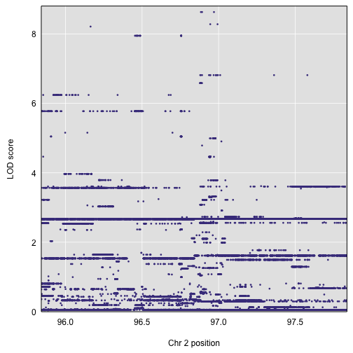
We can use our query_genes() function to identify the genes in the region, and plot_genes() to plot their locations. But also plot_snpasso() can take the gene locations with the argument genes and then display them below the SNP association results. Here, we are also highlighting the top SNPs in the SNP association plot using the drop_hilit argument. SNPs with LOD score within drop_hilit of the maximum are shown in pink.

genes <- query_genes(2, peak_Mbp - 1, peak_Mbp + 1)
par(mar=c(4.1, 4.1, 0.6, 0.6))
plot(out_snps$lod, out_snps$snpinfo, drop_hilit=1.5, genes=genes)

plot of chunk id_and_plot_genes

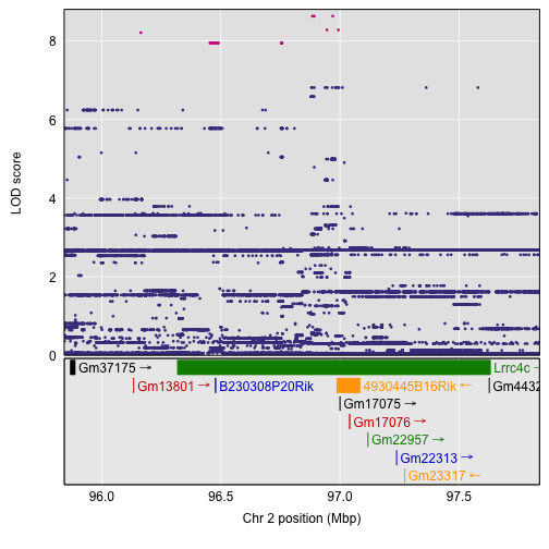
To get a table of the SNPs with the largest LOD scores, use the function top_snps(). This will show all SNPs with LOD score within some amount (the default is 1.5) of the maximum SNP LOD score. We’re going to display just a subset of the columns.

top <- top_snps(out_snps$lod, out_snps$snpinfo)
print(top[,c(1, 8:15, 20)], row.names=FALSE)

                 snp_id A_J C57BL_6J 129S1_SvImJ NOD_ShiLtJ NZO_HlLtJ CAST_EiJ
             rs33297153   1        1           2          1         2        3
            rs226751615   1        1           1          1         2        2
            rs230653109   1        1           1          1         2        2
            rs250407660   1        1           1          1         2        2
            rs248216267   1        1           1          1         2        2
            rs237564299   1        1           1          1         2        2
            rs255011323   1        1           1          1         2        2
            rs212448521   1        1           1          1         2        2
             rs27379206   1        1           1          1         2        2
             rs27379194   1        1           1          1         2        2
            rs244484646   1        1           1          1         2        2
            rs215855380   1        1           1          1         2        2
            rs236942088   1        1           1          1         2        2
            rs212414861   1        1           1          1         2        2
            rs229578122   1        1           1          1         2        2
            rs254318131   1        1           1          1         2        2
            rs217679969   1        1           1          1         2        2
            rs238404461   1        1           1          1         2        2
            rs262749925   1        1           1          1         2        2
            rs231282689   1        1           1          1         2        2
            rs260286709   1        1           1          1         2        2
             rs27396282   1        1           1          1         2        2
            rs263841533   1        1           1          1         2        2
            rs231205920   1        1           1          1         2        2
            rs242885221   1        1           1          1         2        2
            rs586746690   1        1           2          1         2        2
             rs49002164   1        1           2          1         2        2
 SV_2_96945406_96945414   1        1           1          1         2        3
            rs244595995   1        1           2          1         2        2
 SV_2_96993116_96993118   1        1           1          1         2        2
 PWK_PhJ WSB_EiJ      lod
       1       1 8.213182
       1       1 7.949721
       1       1 7.949721
       1       1 7.949721
       1       1 7.949721
       1       1 7.949721
       1       1 7.949721
       1       1 7.949721
       1       1 7.949721
       1       1 7.949721
       1       1 7.949721
       1       1 7.949721
       1       1 7.949721
       1       1 7.949721
       1       1 7.949721
       1       1 7.949721
       1       1 7.949721
       1       1 7.949721
       1       1 7.949721
       1       1 7.949721
       1       1 7.949721
       1       1 7.949721
       1       1 7.949721
       1       1 7.949721
       1       1 7.949721
       1       1 8.631497
       1       1 8.631497
       1       1 8.280942
       1       1 8.631497
       1       1 8.280942

The top SNPs all have NZO and CAST with a common allele, different from the other 6 founders. The next-best SNPs have NZO, CAST, and 129 with a common allele, and then there’s a group of SNPs where NZO has a unique allele.

The scan1snps() function can also be used to perform a genome-wide SNP association scan, by providing a variant query function but leaving chr, start, and end unspecified. In this case it’s maybe best to use keep_all_snps=FALSE (the default) and only save the index SNPs.

out_gwas <- scan1snps(pr, DOex$pmap, DOex$pheno, k, sex, query_func=query_variants, cores=0)

We can make a Manhattan plot of the results as follows. We use altcol to define a color for alternate chromosomes and gap=0 to have no gap between chromosomes.

par(mar=c(4.1, 4.1, 0.6, 0.6))
plot(out_gwas$lod, out_gwas$snpinfo, altcol="green4", gap=0)

plot of chunk plot_gwas_scan

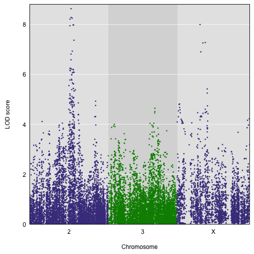
Note that while there are LOD scores on the X chromosome that are as large as those on chromosome 2, we’re allowing a genotype × sex interaction on the X chromosome and so the test has 3 degrees of freedom (versus 2 degrees of freedom on the autosomes) and so the LOD scores will naturally be larger. If we’d used the allele probabilities (apr above, calculated from genoprob_to_alleleprob()) rather than the genotype probabilities, we would be performing a test with 1 degree of freedom on both the X chromosome and the autosomes.

Key Points

SNP association analysis with DO mice requires SNPs in the QTL regions.

.

previous episode

Quantitative Trait Mapping

next episode