Performing a genome scan

Overview

Teaching: 30 min
Exercises: 30 min

Questions

• How do I perform a genome scan?

• How do I plot a genome scan?

Objectives

• Create a genome scan for a set of traits.

• Plot a genome scan.

The freely available chapter on single-QTL analysis from Broman and Sen’s A Guide to QTL Mapping with R/qtl describes different methods for QTL analysis. Two of these methods are described here using data from an experiment on hypertension in the mouse Sugiyama et al., Genomics 71:70-77, 2001. The study employed a backcross between two mouse strains resulting in two possible genotypes - AA for homozygotes, and AB for heterozygotes.

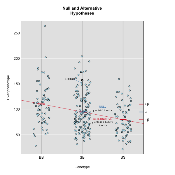
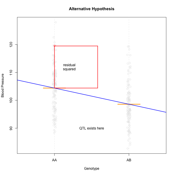
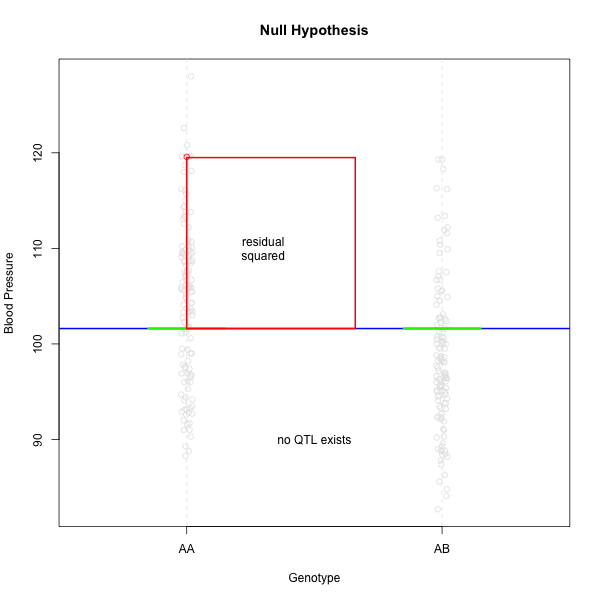
Linear regression can be employed to identify presence of QTL in a cross. To identify QTL using regression, we compare the fit for two models: 1) the null hypothesis that there are no QTL anywhere in the genome; and 2) the alternative hypothesis that there is a QTL near a specific position. A sloped line indicates that there is a difference in mean phenotype between the two genotype groups, and that a QTL is present. A line with no slope indicates that there is no difference in mean phenotype between the two groups, and that no QTL exists. Regression aims to find the line of best fit to the data. In the case of a backcross with only two genotypes, a t-test is performed at the marker to determine whether the difference in phenotype means is zero.

To find the line of best fit, the residuals or errors are calculated, then squared for each data point.

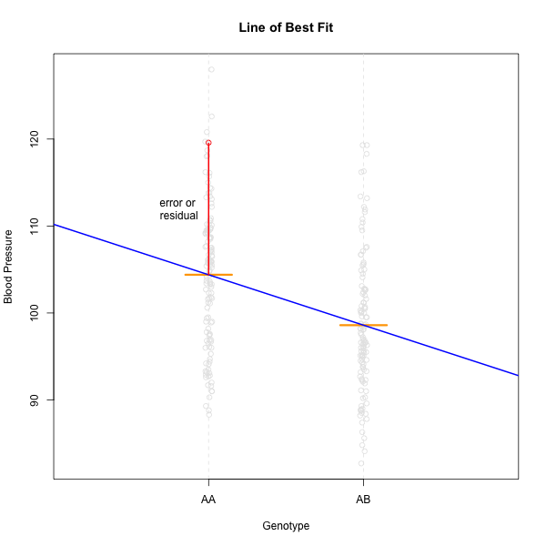
The line of best fit will be the one that minimizes the sum of squared residuals, which maximizes the likelihood of the data.

Marker regression produces a LOD (logarithm of odds) score comparing the null hypothesis to the alternative. The LOD score is calculated using the sum of squared residuals for the null and alternative hypotheses. The LOD score is the difference between the log10 likelihood of the null hypothesis and the log10 likelihood of the alternative hypothesis. It is related to the regression model above by identifying the line of best fit to the data. A higher LOD score indicates greater likelihood of the alternative hypothesis. A LOD score closer to zero favors the null hypothesis.

Marker regression can identify the existence and effect of a QTL by comparing means between groups, however, it requires known marker genotypes and can’t identify QTL in between typed markers. To identify QTL between typed markers, we use Haley-Knott regression. After calculating genotype probabilities, we can regress the phenotypes for animals of unknown genotype on these conditional genotype probabilities (conditional on known marker genotypes). In Haley-Knott regression, phenotype values can be plotted and a regression line drawn through the phenotype mean for the untyped individuals.

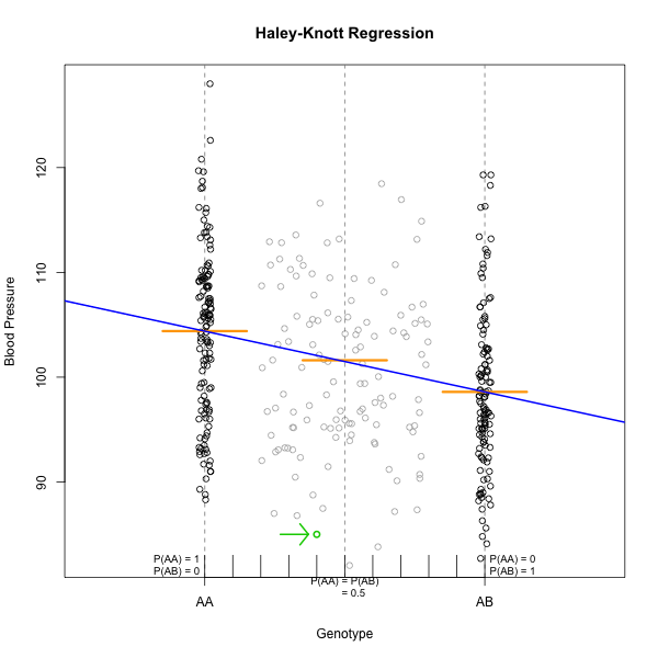
As shown by the green circle in the figure, an individual of unknown genotype is placed between known genotypes according to the probability of its genotype being AA or AB. In this case, the probability of this individual having genotype AA is 0.6, and the probability of having genotype AB is 0.4.

To perform a genome scan by Haley-Knott regression (Haley and Knott 1992), use the function scan1(). scan1() takes as input the genotype probabilities, a matrix of phenotypes, and then optional additive and interactive covariates, and the special X chromosome covariates. Another option is to provide a vector of weights.

out <- scan1(genoprobs = pr, pheno = iron$pheno, Xcovar=Xcovar)

On a multi-core machine, you can get some speed-up via the cores argument, as with calc_genoprob() and calc_kinship().

out <- scan1(genoprobs = pr, pheno = iron$pheno, Xcovar=Xcovar, cores=4)

The output of scan1() is a matrix of LOD scores, positions × phenotypes.

Take a look at the first ten rows of the scan object. The numerical values are the LOD scores for the marker or pseudomarker named at the beginning of the row. LOD values are given for liver and spleen.

head(out, n=10)

             liver    spleen
D1Mit18  0.2928511 0.4566189
c1.loc28 0.2815294 0.4378754
c1.loc29 0.2696594 0.4193363
c1.loc30 0.2572780 0.4011646
c1.loc31 0.2444340 0.3835257
c1.loc32 0.2311884 0.3665798
c1.loc33 0.2176149 0.3504744
c1.loc34 0.2037988 0.3353358
c1.loc35 0.1898359 0.3212614
c1.loc36 0.1758305 0.3083145

The function plot_scan1() can be used to plot the LOD curves. Use the argument lodcolumn to indicate which column to plot.

plot_scan1(out, map = map, lodcolumn = "liver")

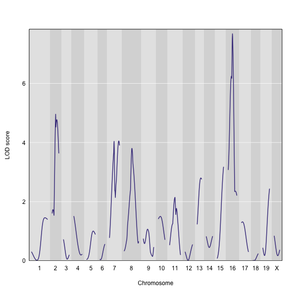
The LOD plot for liver clearly shows the largest peak is on chromosome 16. There are smaller peaks on chromosomes 2, 7, and 8. Which of these peaks is significant, and why? We’ll evaluate the significance of genome scan results in a later episode on performing a permutation test.

Challenge 1

Use the head() function to view the first 30 rows of the scan output. What is the next genotyped marker in the scan output? What are its LOD scores for liver and spleen?

Solution to Challenge 1

head(out, n=30)
D1Mit80 0.02154502 0.2216682

Challenge 2

Use the sort() function to sort the LOD scores for liver. Hint: run dim(out) for the row and column dimensions, or colnames(out) for the column names.
Which pseudomarker has the highest LOD score? Which genotyped marker has the highest LOD score? What chromosome number are they on?

Solution to Challenge 2

sort(out[,1]) for column 1 or sort(out[,"liver"]) for the column named “liver”.
The pseudomarker with the largest score is c16.loc29, with a LOD of 7.68. The genotyped marker with the largest LOD is D16Mit30 with a score of 7.28. Both are located on chromosome 16.

Challenge 3

Use the sort() function to sort the LOD scores for spleen. Which pseudomarker has the highest LOD score? Which genotyped marker has the highest LOD score? What chromosome number are they on?

Solution to Challenge 3

sort(out[,2]) or sort(out[,"spleen"]) The pseudomarker with the largest score is c9.loc57, with a LOD of 12.1. The genotyped marker with the largest LOD is D9Mit182 with a score of 10.4. Both are located on chromosome 9.

Challenge 4

Plot the LOD scores for spleen. Does the genome scan for spleen share any large-ish peaks with the scan for liver?

Solution to Challenge 4

plot_scan1(out, map = map, lodcolumn = "spleen") Both liver and spleen genome scans share a peak on chromosome 8 with a LOD score near 4.

Key Points

• A qtl2 genome scan requires genotype probabilities and a phenotype matrix.

• The output from a genome scan contains a LOD score matrix, map positions, and phenotypes.

• LOD curve plots for a genome scan can be viewed with plot_scan1().