Calculating A Kinship Matrix
Overview
Teaching: 30 min
Exercises: 30 minQuestions
Why would I calculate kinship between individuals?
How do I calculate kinship between individuals?
What does a kinship matrix look like?
Objectives
Explain why and when kinship calculation matters in mapping.
Create a kinship matrix for individuals.
Population structure and kinship are common confounding factors in genome-wide association studies (GWAS), case-control studies, and other study types in genetics. They create false positive associations between genotype and phenotype at genetic markers that differ in genotype frequencies between subpopulations due to genetic relatedness between samples. Simple association tests assume statistical independence between individuals. Population structure and kinship confound associations when phenotype covariance between individuals results from genetic similarity. Accounting for relatedness between individuals helps to distinguish true associations from false positives generated by population structure or kinship.
As an example see the table below for phenotype and genotype frequencies between two subpopulations in a case-control study.
| subpop1 | subpop2 | overall pop | |
|---|---|---|---|
| frequency | 0.5 | 0.5 | 1 |
| probability of AA genotype | 0.1 | 0.9 | 0.5 |
| probability of disease | 0.9 | 0.1 | 0.5 |
| probability of disease & AA | 0.09 | 0.09 | 0.09 |
The full population consists of two equally represented subpopulations. In the overall population, the probability of the AA genotype is 0.5, and the probability of disease is also 0.5. The joint probability of both disease and AA genotype in the population (0.09) is less than either the probability of disease (0.5) or the probability of the AA genotype (0.5) alone, and is considerably less than the joint probability of 0.25 that would be calculated if subpopulations weren’t taken into account. In a case-control study that fails to recognize subpopulations, most of the cases will come from subpopulation 1 since this subpopulation has a disease probability of 0.9. However, this subpopulation also has a low probability of the AA genotype. So a false association between AA genotype and disease would occur because only overall population probabilities would be considered.
Linear mixed models (LMMs) consider genome-wide similarity between all pairs of individuals to account for population structure, known kinship and unknown relatedness. They model the covariance between individuals. Linear mixed models in association mapping studies can successfully correct for genetic relatedness between individuals in a population by incorporating kinship into the model. To perform a genome scan by a linear mixed model, accounting for the relationships among individuals (in other words, including a random polygenic effect), you’ll need to calculate a kinship matrix for the individuals. This is accomplished with the calc_kinship() function. It takes the genotype probabilities as input.
kinship <- calc_kinship(probs = pr)
Take a look at the kinship values calculated for the first 5 individuals.
kinship[1:5, 1:5]
          1         2         3         4         5
1 0.6780378 0.5070425 0.4770823 0.5100762 0.5193062
2 0.5070425 0.5612483 0.5139017 0.4777593 0.5049052
3 0.4770823 0.5139017 0.7272491 0.5147456 0.5393396
4 0.5100762 0.4777593 0.5147456 0.7153455 0.5359428
5 0.5193062 0.5049052 0.5393396 0.5359428 0.5775571
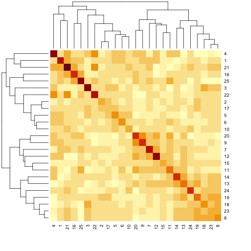
We can also look at the first 50 mice in the kinship matrix.
n_samples <- 25
heatmap(kinship[1:n_samples, 1:n_samples], symm = TRUE)

The mice are listed in the same order on both sides of the matrix. The comb-like structures are called “dendrograms” and they indicate how the mice are clustered together. Each cell represents the degree of allele sharing between mice. Red colors indicate higher kinship and yellow colors indicate lower kinship. Each mouse is closely related to itself, so the cells along the diagonal tend to be darker than the other cells. You can see some evidence of related mice, possibly siblings, in the orange-shaded blocks along the diagonal.
By default, the genotype probabilities are converted to allele probabilities, and the kinship matrix is calculated as the proportion of shared alleles. To use genotype probabilities instead, use use_allele_probs=FALSE in the call to calc_kinship(). Further, by default we omit the X chromosome and only use the autosomes. To include the X chromosome, use omit_x=FALSE.
In calculating the kinship matrix, you can eliminate the effect of varying marker density across the genome, and only use the probabilities along the grid of pseudomarkers (defined by the step argument to insert_pseudomarkers(). To do so, we need to first use calc_grid() to determine the grid of pseudomarkers, and then probs_to_grid() to probabilities for positions that are not on the grid.
grid <- calc_grid(map = iron$gmap, step=1)
pr_grid <- probs_to_grid(probs = pr, grid = grid)
kinship_grid <- calc_kinship(probs = pr_grid)
On a multi-core machine, you can get some speed-up via the cores argument, as with calc_genoprob().
kinship <- calc_kinship(pr, cores=4)
Challenge 1
1). Insert pseudomarkers into a new map called
sparser_mapat 2 cM intervals.
2). Calculate genotype probabilities and save as an object calledpr2. Leave the error probability at the default value.
3). Calculate kinship with these new probabilities. Save askinship2.
4). View the first several rows and columns of thekinship2matrix and compare to the originalkinshipmatrix with a heatmap.Solution to Challenge 1
1).
sparser_map <- insert_pseudomarkers(map = map, step = 2)
2).pr2 <- calc_genoprob(cross = iron, map = sparser_map)
3).kinship2 <- calc_kinship(probs = pr2)
4).kinship2[1:5, 1:5]andheatmap(kinship2[1:n_samples, 1:n_samples], symm = TRUE)
Challenge 2
Think about what a kinship matrix is and what it represents. Share your understanding with a neighbor. Write your explanation in the collaborative document or in your own personal notes.
Solution to Challenge 2
Key Points
Kinship matrices account for relationships among individuals.
Kinship is calculated as the proportion of shared alleles between individuals.
Kinship calculation is a precursor to a genome scan via a linear mixed model.