Estimating QTL effects
Last updated on 2025-10-07 | Edit this page
Overview
Questions
- How do I find the founder allele effects at a QTL peak?
Objectives
- Estimate the founder allele effects at a QTL peak.
- Plot the estimated founder allele effects.
Estimating Founder Allele Effects
Recall that to model data from a cross, we use
\(y_j = \mu + \beta_k G_{jk} + \epsilon_j\)
where \(y_{ij}\) is the phenotype of the \(j\)th individual, \(\mu\) is the mean phenotype value, \(\beta_k\) is the effect of the \(k\)th genotype, \(G_{jk}\) is the genotype for individual \(j\), and \(\epsilon_j\) is the error for the \(j\)th individual. In the figure below, \(\mu\) equals 94.6 and \(\beta\) equals 15 for the alternative hypothesis (QTL exists).
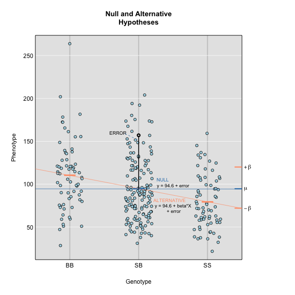
This linear model is \(y\) = 94.6 + 15\(G\) + \(\epsilon\). The model intersects the genotype groups at their group means, and is based \(\mu\) and \(\beta_k\).
The effect of genotype RR (the \(\beta\) for the RR genotype) at the marker is 15, while the effect of the BB genotype is -15 on the phenotype. The effect of the BR genotype is 0 relative to \(\mu\) equals 94.6.
The scan1() function returns only LOD scores. To obtain
estimated QTL effects, use the function scan1coef(). This
function takes a single phenotype and the genotype probabilities for a
single chromosome and returns a matrix with the estimated coefficients
at each putative QTL location along the chromosome.
For example, to get the estimated QTL effects on chromosome 19 for
the insulin phenotype, we would provide the chromosome 19 genotype
probabilities and the insulin phenotype to the function
scan1coef() as follows:
R
chr       <- "19"
eff_chr19 <- scan1coef(genoprobs = probs[,chr],
                       pheno     = insulin,
                       kinship   = kinship_loco[[chr]],
                       addcovar  = addcovar)
The result is a matrix of 50 positions \(\times\) 3 genotypes. Additional columns contain the sex and intercept values (\(\mu\)).
R
head(eff_chr19)
OUTPUT
                BB      BR     RR SexMale intercept
rs4232073  -0.0387 -0.0275 0.0661  -0.169      1.01
rs13483548 -0.0386 -0.0272 0.0658  -0.168      1.01
rs13483549 -0.0388 -0.0272 0.0660  -0.169      1.01
rs13483550 -0.0413 -0.0275 0.0688  -0.169      1.01
rs13483554 -0.0374 -0.0325 0.0698  -0.170      1.01
rs13483555 -0.0367 -0.0288 0.0655  -0.170      1.01
Plotting Founder Allele Effects Along a Chromosome
To plot the QTL effects, use the plot_coef() function.
Add the LOD plot to the scan1_output argument to include a
LOD plot at the bottom.
R
plot_coef(x            = eff_chr19,
          map          = cross$pmap,
          scan1_output = lod_add_loco,
          legend       = "topleft")
The plot shows effect values on the y-axis and cM values on the x-axis. The value of the intercept (\(\mu\)) appears at the top. The effect of the BR genotype is centered around zero, with the effects of the other two genotypes above and below. We are usually not directly interested in how the additive covariates change across the genome, but rather, how the founder allele effects change.
To plot only the founder allele effects, use the argument
columns to indicate which coefficients to plot. Let’s look
at the columns which contain the founder allele effects.
R
head(eff_chr19)
OUTPUT
                BB      BR     RR SexMale intercept
rs4232073  -0.0387 -0.0275 0.0661  -0.169      1.01
rs13483548 -0.0386 -0.0272 0.0658  -0.168      1.01
rs13483549 -0.0388 -0.0272 0.0660  -0.169      1.01
rs13483550 -0.0413 -0.0275 0.0688  -0.169      1.01
rs13483554 -0.0374 -0.0325 0.0698  -0.170      1.01
rs13483555 -0.0367 -0.0288 0.0655  -0.170      1.01
We would like to plot the columns “BB”, “BR”, and “RR”, which are in
columns 1 through 3. This is what we pass into the columns
argument.
R
plot_coef(x = eff_chr19,
map = cross$pmap,
columns = 1:3,
scan1_output = lod_add_loco,
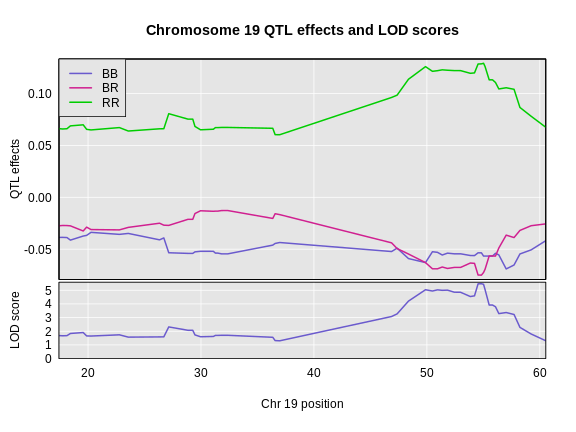
main = paste("Chromosome", chr, "QTL effects and LOD scores"),
legend = "topleft")
Challenge 1: Founder Allele Effects
Looking at the plot above, which founder allele contributes to higher insulin levels?
The BTBR allele contributes to higher insulin levels because the “RR” allele effect (green line) is higher than the other allele effect lines.
Estimating Founder Allele Effects using BLUPs
Another option for estimating the founder allele effects is to treat
them as random
effects and calculate Best
Linear Unbiased Predictors (BLUPs). This is particularly valuable
for multi-parent populations such as the Collaborative Cross and
Diversity Outbred mice, where the large number of possible genotypes at
a QTL leads to considerable variability in the effect estimates. To
calculate BLUPs, use scan1blup(); it takes the same
arguments as scan1coef(), including the option of a kinship
matrix to account for a residual polygenic effect.
R
blup_chr19 <- scan1blup(genoprobs = probs[,chr],
                        pheno     = insulin,
                        kinship   = kinship_loco[[chr]],
                        addcovar  = addcovar)
We can plot the BLUP effects using plot_coef as
before.
R
plot_coef(x       = blup_chr19,
          map     = cross$pmap,
          columns = 1:3,
          scan1_output = lod_add_loco,
          main    = paste("Chromosome", chr, "QTL BLUP effects and LOD scores"),
          legend  = "topleft")
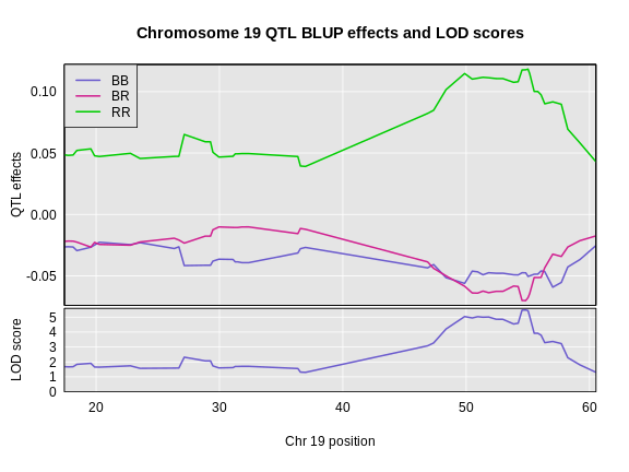
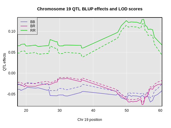
In the plot below, we plotted the founder allele effects (solid lines) and the BLUPs (dashed lines). In this case, the effects are not greatly different, but the effects are “shrunken” toward zero.
R
plot_coef(x       = eff_chr19,
          map     = cross$pmap,
          columns = 1:3,
          main    = paste("Chromosome", chr, "QTL BLUP effects and LOD scores"),
          legend  = "topleft")
plot_coef(x       = blup_chr19,
          map     = cross$pmap,
          columns = 1:3,
          lty     = 2,
          legend  = "topleft",
          add     = TRUE)
Plotting Allele Effects at One Marker
You may also want plot the founder allele effects at the marker with the highest LOD. To do this, you first need to get the position of the marker from the peak list.
R
peaks <- find_peaks(scan1_output = lod_add_loco,
                    map          = cross$pmap,
                    threshold    = thr)
peaks
OUTPUT
  lodindex          lodcolumn chr   pos  lod
1        1 log10_insulin_10wk   2 138.9 7.13
2        1 log10_insulin_10wk   7 144.2 5.72
3        1 log10_insulin_10wk  12  25.1 4.31
4        1 log10_insulin_10wk  14  22.2 3.97
5        1 log10_insulin_10wk  16  80.4 4.11
6        1 log10_insulin_10wk  19  54.8 5.48
The position of the maximum LOD on chromosome 19 is 54.83 Mb. We can
pass this value into the qtl2 function
pull_genoprobpos to get the genoprobs at this marker.
R
max_pos <- subset(peaks, chr == '19')$pos
max_mkr <- find_marker(map = cross$pmap,
                       chr = chr,
                       pos = max_pos)

pr      <- pull_genoprobpos(genoprobs = probs,
                            marker    = max_mkr)
Challenge 2: Structure of Genoprobs at One Marker
What does the structure of pr look like? How many rows
and columns does it have?
The str function provides the structure of an R object.
R
str(pr)
OUTPUT
 num [1:490, 1:3] 1.09e-08 1.09e-08 3.06e-14 1.09e-08 1.09e-08 ...
 - attr(*, "dimnames")=List of 2
  ..$ : chr [1:490] "Mouse3051" "Mouse3551" "Mouse3430" "Mouse3476" ...
  ..$ : chr [1:3] "BB" "BR" "RR"
In this case, we can see that pr is a numeric matrix
because the first line starts with “num”. The next item on the first
line provides the dimensions of the object. pr is a matrix
because there are two dimensions, rows and columns. There are 490 rows
and 3 columns in pr.
Challenge 3: Genoprobs at One Marker
Look at the top few rows of pr. You may want to round
the values to make them easier to read. What is the genotype of
Mouse3051? What about Mouse3430?
We can use the head function to see the top few rows
of pr.
R
head(round(pr))
OUTPUT
          BB BR RR
Mouse3051  0  1  0
Mouse3551  0  1  0
Mouse3430  0  0  1
Mouse3476  0  1  0
Mouse3414  0  1  0
Mouse3145  0  1  0
From the listing above, the probability that Mouse3051 carries the “BR” genotype at this marker is close to 1, so this is the most likely genotype.
the probability that Mouse3430 carries the “RR” genotype at this marker is close to 1.
pr is a numeric matrix with 490 rows and 3 columns. The
rownames contain the mouse IDs and the column names contain the
genotypes.
We can then pass pr as an argument into the
fit1 function, which fits the mapping model at a single
marker.
R
mod = fit1(genoprobs = pr,
           pheno     = insulin,
           kinship   = kinship_loco[[chr]],
           addcovar  = addcovar)
Then, we can plot the founder allele effects and their standard error.
R
mod_eff = data.frame(eff = mod$coef,
                     se  = mod$SE) |>
           rownames_to_column("genotype") |>
           filter(genotype %in% c("BB", "BR", "RR"))

ggplot(data    = mod_eff,
       mapping = aes(x = genotype, y = eff)) +
  geom_pointrange(mapping = aes(ymin = eff - se,
                                ymax = eff + se),
                  size       = 1.5,
                  linewidth  = 1.25) +
  labs(title = paste("Founder Allele Effects on Chr", chr),
       x     = "Genotype", y = "Founder Allele Effects") +
  theme(text = element_text(size = 20))
 ::::::::::::::::::::::::::::::::::::: challenge
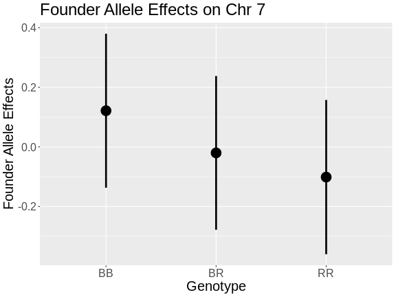
Challenge 4: Allele Effects
- In the plot above, which founder allele contributes to higher insulin levels?
- Is that consistent with the plot created using
plot_coefabove?
- The R (BTBR) allele contributes to higher insulin levels on chromosome 19.
- Yes, the BTBR allele also contributed to higher insulin level in the founder allele effects plot.
Challenge 5: Allele Effects on Chromosome 7
- Use
scan1_blupandplot_coefto look at the founder allele effects at the chromosome 7 QTL peak. Does the pattern of allele effects look different? Which founder allele contributes to higher insulin levels? - Get the genoprobs at the marker with the highest LOD on chromosome 7
and use
fit1and the plotting code forfit1above to examine the founder allele effects at the peak marker. Again, how do these allele effects differ from the allele effects on chromosome 19? Which founder allele contributes to higher insulin levels?
Be careful to rename the ouput objects so that you don’t overwrite the values from chromosome 19.
- We will use
scan1_blupandplot_coefto estimate the founder allele effects on chromosome 7.
R
blup_chr7 <- scan1blup(genoprobs = probs[,"7"],
                       pheno     = insulin,
                       kinship   = kinship_loco[["7"]],
                       addcovar  = addcovar)
plot_coef(x       = blup_chr7,
          map     = cross$pmap,
          columns = 1:3,
          scan1_output = lod_add_loco,
          main    = paste("Chromosome", "7", "QTL BLUP effects and LOD scores"),
          legend  = "topleft")
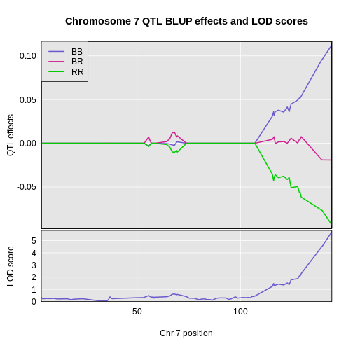
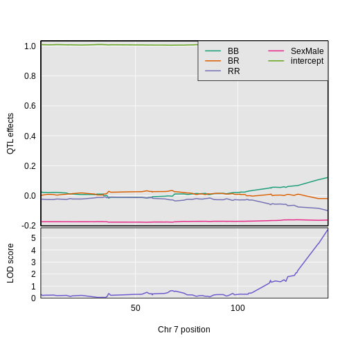
On chromosome 19, the BB and BR genotypes seems to have the same effect. On chromosome 7, there is a clear split between the BB, BR, and RR genotypes. Each additional B allele raises insulin levels. The C57BL/6J (B) allele contributes to higher insulin levels.
- We will get the marker with the highest LOD on chromosome 7, then
get the genoprobs at that marker and use them in
fit1to estimate the founder allele effects.
R
max_pos <- subset(peaks, chr == "7")$pos
max_mkr <- find_marker(map = cross$pmap,
                       chr = "7",
                       pos = max_pos)

pr7     <- pull_genoprobpos(genoprobs = probs,
                            marker    = max_mkr)
R
mod7 = fit1(genoprobs = pr7,
            pheno     = insulin,
            kinship   = kinship_loco[["7"]],
            addcovar  = addcovar)
R
mod_eff7 = data.frame(eff = mod7$coef,
                      se  = mod7$SE) |>
            rownames_to_column("genotype") |>
            filter(genotype %in% c("BB", "BR", "RR"))

ggplot(data    = mod_eff7,
       mapping = aes(x = genotype, y = eff)) +
  geom_pointrange(mapping = aes(ymin = eff - se,
                                ymax = eff + se),
                  size       = 1.5,
                  linewidth  = 1.25) +
  labs(title = paste("Founder Allele Effects on Chr", "7"),
       x     = "Genotype", y = "Founder Allele Effects") +
  theme(text = element_text(size = 20))
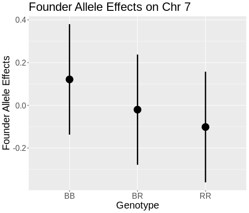
On chromosome 19, mice carrying the BB and BR genotypes had almost the same levels of insulin. On chromosome 7, the BB genotype has the highest insulin levels, the BR genotype has the next highest, and the RR genotype has the lowest insulin levels.
::::::::::::::::::::::::::::::::::::::::::::::::
Estimating Additive and Dominant Allele Effects
You may have noticed the difference in the pattern of allele effects between chromosome 7 and 19. On chromosome 7, adding each “B” allele increased insulin levels by the same amount. On chromosome 19, adding one “R” allele did not change insulin levels. We saw an increase in insulin only when we added two “R” alleles.
What we are seeing between these two QTL are “additive” and “dominant” effects. At an additive QTL (which is different from additive covariates), adding (or subtracting) one allele produces the same effect between each genotype. At a dominant QTL, adding (or subtracting) two alleles is required to see the effect. You can also have QTL which are a mixture of additive and dominant effects.
We can map the additive and dominance effects by providing a matrix of contrasts to indicate the different effects. Let’s look at the additive and dominant effects on chromosome 7 first.
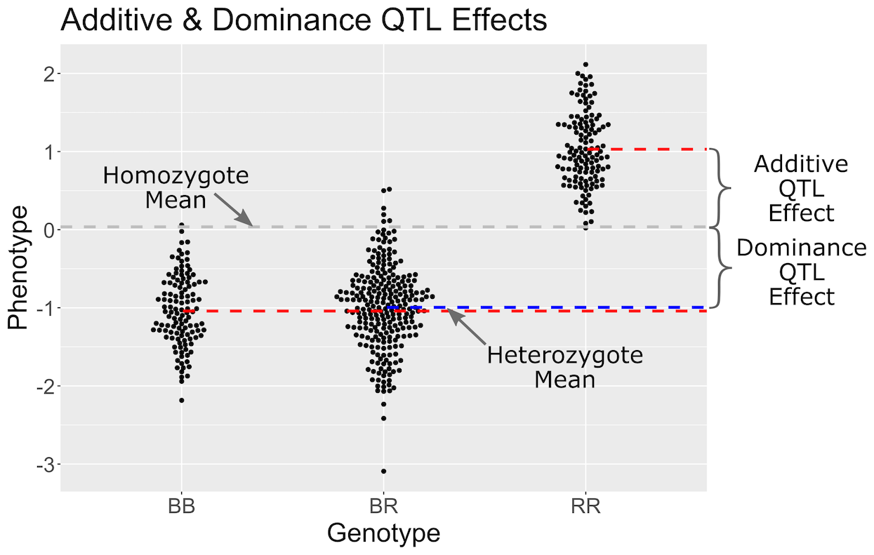
In the figure above, we have simulated a QTL with a dominant effect. Genotypes are shown on the X-axis and the phenotype on the Y-axis. Each point represents the phenotype value for one mouse. The grey line is the mean of the two homozygote groups. The additive effect is defined as the difference between the homozygote mean (grey line) and the individual homozygote group means (red lines). The blue line shows the heterozygote mean. The dominance effect is the difference between the homozygote mean (grey line) and the heterozygote mean (blue line).
First, we create a contrasts matrix to indicate the mean, additive, and dominance effects that we want to estimate.
R
add_dom_contr <- cbind(mu = c( 1, 1, 1),
                       a  = c(-1, 0, 1),
                       d  = c( 0, 1, 0))
R
c7effB <- scan1coef(genoprobs = probs[,"7"],
                    pheno     = insulin,
                    kinship   = kinship_loco[["7"]],
                    addcovar  = addcovar,
                    contrasts = add_dom_contr)
The result will then contain the estimates of mu,
a (the additive effect), and d (the dominance
effect).
R
dim(c7effB)
OUTPUT
[1] 109 4R
head(c7effB)
OUTPUT
             mu       a        d SexMale
rs8252589  1.01 -0.0267 -0.00378  -0.175
rs13479104 1.01 -0.0228  0.00409  -0.175
rs13479112 1.01 -0.0234  0.00991  -0.175
rs13479114 1.00 -0.0226  0.01148  -0.175
rs13479120 1.01 -0.0238  0.00899  -0.175
rs13479124 1.01 -0.0219  0.00375  -0.175
For marker rs13479570, mu, a, and
d are 1.016, -0.111, -0.03, -0.164.
Here’s a plot of the chromosome 7 additive and dominance effects, which are in the second and third columns.
R
plot_coef(x       = c7effB,
          map     = cross$pmap["7"],
          columns = 2:3,
          col     = 1:2,
          scan1_output = lod_add_loco,
          main    = "log10(insulin): Chromosome 7")
legend('bottomleft', lwd = 2, col = 1:2, legend = c("additive", "dominance"))
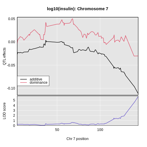
In the plot above, the dominance effects remain near zero across the chromosome. The additive effects decrease as we move
Challenge 6: Estimating Additive and Dominance Effects on Chromsome 19
Use the code above to estimate and plot the additive and dominance effects along chromosome 19. You can use the same contrasts matrix as before. How dow they differ from the effects on chromosome 7?
First we estimate the effects using scan1coef.
R
c19effB <- scan1coef(genoprobs = probs[,"19"],
                     pheno     = insulin,
                     kinship   = kinship_loco[["19"]],
                     addcovar  = addcovar,
                     contrasts = add_dom_contr)
R
plot_coef(x       = c19effB,
          map     = cross$pmap["19"],
          columns = 2:3,
          col     = c("black", "red"),
          scan1_output = lod_add_loco,
          main    = "log10(insulin): Chromosome 19")
legend('bottomleft', lwd = 2, col = c("black", "red"),
       legend = c("additive", "dominance"))
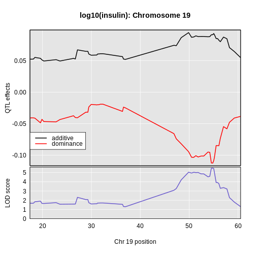
In this case, we see that the additive effect adds about 0.094 and the dominance effect adds about -0.113.
Plotting Phenotypes versus Genotypes
Finally, to plot the raw phenotypes against the genotypes at a single
putative QTL position, you can use the function plot_pxg().
This takes a vector of genotypes as produced by the
maxmarg() function, which picks the most likely genotype
from a set of genotype probabilities, provided it is greater than some
specified value (the argument minprob). Note that the
marg in maxmarg stands for “marginal”, as this
function is selecting the genotype at each position that has maximum
marginal probability.
For example, we could get inferred genotypes at the chr 19 QTL for the insulin phenotype (at 28.6 cM) as follows:
R
g <- maxmarg(probs = probs,
             map   = cross$pmap,
             chr   = chr,
             pos   = max_pos,
             return_char = TRUE)
We use return_char = TRUE to have maxmarg()
return a vector of character strings with the genotype labels.
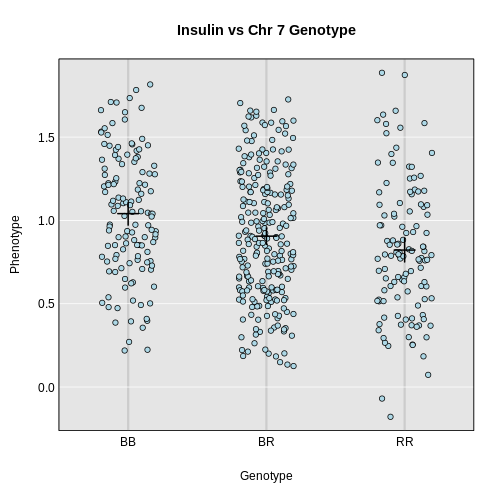
We then plot the insulin phenotype against these genotypes as follows:
R
plot_pxg(geno   = g,
         pheno  = insulin,
         SEmult = 2,
         main   = paste("Insulin vs Chr", chr ,"Genotype"))
- Estimated founder allele effects can be plotted from the mapping model coefficients.
- Additive and dominance effects can be plotted using contrasts.