Integrating Gene Expression Data
Last updated on 2025-10-07 | Edit this page
Overview
Questions
- How can I use gene expression data to identify candidate genes?
- What is expression QTL mapping?
Objectives
- Find genes which are correlated with a physiological phenotype.
- Find genes which have expression QTL in the same position as a physiological phenotype.
Introduction
Once you have QTL peak, the next step if often to identify genes which may be causal candidates. However, there are often hundreds of genes within the QTL support interval. How do you select candidate genes?
Often, there is a tissue which is related to the phenotype that you are measuring. For example, if you measure circulating cardiac troponin, then gene expression in the heart may be relevant. For some complex phenotypes, it may not be easy to select a tissue. For example, if the liver creates a metabolite that causes kidney injury, which is then exacerbated by the immune system, in which tissue would you measure gene expression?
Susceptibility to type 2 diabetes involves a complex interaction between several tissues. However, for the purposes of this tutorial in which we mapped circulating insulin levels, it is reasonable to look at gene expression in the pancreas.
Reading in Gene Expression Data
Gene expression data consists of two parts: expression measurements and gene annotation. In this study, gene expression was measured via two-color microarray. The expression values represent a ratio of two sets of RNA: a control set and the sample set. The expression values represent the log-normalized ratio of these two sets.
We have prepared two files containing normalized gene expression data and the gene annotation.
R
annot <- read_csv("data/attie_b6btbr_grcm39/attie_gene_annot.csv",
                  show_col_types = FALSE) |>
           mutate(a_gene_id = as.character(a_gene_id))

expr  <- read_csv("data/attie_b6btbr_grcm39/attie_gene_expr.csv",
                  show_col_types = FALSE)
Challenge 1: Size of data structures.
- How many rows and columns are in
annot? - What are the column names off
annot?
Dimensions of annot.
R
dim(annot)
OUTPUT
[1] 29860 13Column names of annot.
R
colnames(annot)
OUTPUT
 [1] "a_gene_id"       "chr"             "start"           "end"
 [5] "width"           "strand"          "gene_id"         "gene_name"
 [9] "gene_biotype"    "description"     "gene_id_version" "symbol"
[13] "entrezid"
Challenge 2
- What are the dimensions of
expr? - Look at the top 5 row by 5 column block of
expr.
- Dimensions of
expr.
R
dim(expr)
OUTPUT
[1] 490 29861- Top-left block of
expr.
R
expr[1:5,1:5]
OUTPUT
# A tibble: 5 × 5
  MouseNum  `497628` `497629` `497630` `497632`
  <chr>        <dbl>    <dbl>    <dbl>    <dbl>
1 Mouse3051  -0.0790 -0.0114  -0.0790    0.0461
2 Mouse3551   0.0544 -0.0693  -0.0721   -0.408
3 Mouse3430   0.154  -0.0468  -0.00900  -0.298
4 Mouse3476   0.144  -0.0451  -0.00505   0.12
5 Mouse3414   0.266   0.00496 -0.0746   -0.127
Let’s look at the relationship between the annotation and the expression data.
The annotation data has 29860 rows and the expression data has 29861
columns. The first column in expr contains the mouse ID and
the remaining columns contain the expression values for each gene. The
gene IDs are in the column names. These are Agilent gene IDs. They are
also in the a_gene_id column in the annotation.
R
all(annot$a_gene_id == colnames(expr)[-1])
OUTPUT
[1] TRUENow we know that the genes are aligned between the annotation and the expression data. When you receive your own expression data, it is critical that you align the genes in your expression data with your annotation data.
We must also align the mouse IDs between the physiological phenotypes and the expression data. We saw above that the mouse IDs are in the first column of the expression data. Let’s see where the mouse IDs are in the phenotype data.
R
head(cross$pheno)
OUTPUT
          log10_insulin_10wk agouti_tan tufted
Mouse3051              1.399          1      0
Mouse3551              0.369          1      1
Mouse3430              0.860          0      1
Mouse3476              0.800          1      0
Mouse3414              1.370          0      0
Mouse3145              1.783          1      0
cross$pheno is a matrix which contains the mouse IDs in
the rownames. Let’s convert the expression data to a matrix as well.
R
expr <- expr |>
         column_to_rownames(var = "MouseNum") |>
         as.matrix()
Now let’s check whether the mouse IDs are aligned between
cross$pheno and expr. Again, when you assemble
your phenotype and expression data, you will need to make sure that the
sample IDs are aligned between the data sets.
R
all(rownames(cross$pheno) == rownames(expr))
OUTPUT
[1] TRUEIdentifying Genes in a QTL Support Interval
In previous episodes, we found significant QTL peaks using the
find_peaks function. Let’s look at those peaks again.
R
peaks
OUTPUT
  lodindex          lodcolumn chr   pos  lod  ci_lo ci_hi
1        1 log10_insulin_10wk   2 138.9 7.13  64.95 149.6
2        1 log10_insulin_10wk   7 144.2 5.72 139.37 144.2
3        1 log10_insulin_10wk  12  25.1 4.31  15.83  29.1
4        1 log10_insulin_10wk  14  22.2 3.97   6.24  45.9
5        1 log10_insulin_10wk  16  80.4 4.11  10.24  80.4
6        1 log10_insulin_10wk  19  54.8 5.48  48.37  55.2
We looked at the QTL peak on chromosome 19 in a previous lesson. The QTL interval is 6.779 Mb wide. This is quite wide. Let’s get the genes expressed in the pancreas within this region.
R
chr         <- '19'
peaks_chr19 <- filter(peaks, chr == '19')
annot_chr19 <- filter(annot, chr == '19' & start > peaks_chr19$ci_lo & end < peaks_chr19$ci_hi)
expr_chr19  <- expr[,annot_chr19$a_gene_id]
There are 22 genes! How can we start to narrow down which ones may be candidate genes?
Challenge 3: How can we narrow down the candidate gene list?
- Take a moment to think of ways that you could narrow down the gene list to select the most promising candidate genes that regulate insulin levels.
- Turn to your neighbor and exchange your ideas.
- Share your ideas with the group.
Identifying Coding SNPs in QTL Intervals
When you have a QTL peak, you can search for SNPs which lie within the coding regions of genes. These SNPs may cause amino acid substitutions which will affect protein structure. The most comprehensive SNP resource is the Mouse Genomes Project. They have sequenced 52 inbred strains, including BTBR, and have made the data available in Variant Call Format (VCF). The full VCF files are available on the EBI FTP site. However, the full SNP file is 22 GB! When you need other strains, you can download and query that file. However, for this workshop, we only need SNPs for the BTBR strain. We have created a VCF file containing only SNPs which differ from C57BL/6J and BTBR. Let’s read in this file now using the VariantAnnotation function readVcf.
R
vcf <- readVcf(file.path("data", "btbr_snps_grcm39.vcf.gz"))
The vcf object contains both the SNP allele calls and
information about the sequencing depth and SNP consequences. Let’s see
how many SNPs are in the VCF.
R
dim(vcf)
OUTPUT
[1] 4791000 1There are about 4.8 million SNPs in vcf. There are many
fields in the VCF file and there are vignettes
which document the more advanced features. Here, we will search for SNPs
within QTL support intervals and filter them to retain missense or stop
coding SNPs.
In order to filter the SNPs by location, we need to create a GenomicRanges
object which contains the coordinates of the QTL support interval on
chromosome 19. Note that the support interval is reported by
qtl2 in Mb and the GRanges object must be given bp
positions, so we need to multiply these by 1e6.
R
chr19_gr <- GRanges(seqnames = peaks_chr19$chr,
                    ranges   = IRanges(peaks_chr19$ci_lo * 1e6, peaks_chr19$ci_hi * 1e6))
chr19_gr
OUTPUT
GRanges object with 1 range and 0 metadata columns:
      seqnames            ranges strand
         <Rle>         <IRanges>  <Rle>
  [1]       19 48370979-55150074      *
  -------
  seqinfo: 20 sequences from an unspecified genome; no seqlengths
Next, we will filter the vcf object to retain SNPs
within the support interval.
R
vcf_chr19 <- subsetByOverlaps(vcf, ranges = chr19_gr)
Let’s see how many SNPs there are.
R
dim(vcf_chr19)
OUTPUT
[1] 19065 1There are still 19,000 SNPs! But many of them may not be in coding regions or may be synonymous. Next, we will search for SNPs that have missense or stop coding changes. These are likely to have the most severe effects. Note that synonymous SNPs and SNPs in the untranslated region of genes may affect RNA folding, RNA stability, and translation. But it is more difficult to predict those effects.
Let’s plot the density of the SNPs to see where they fall. We would not expect genes which lie in regions without variation between B6 and BTBR to be involved in regulating insulin levels.
R
# Get the SNP positions.
pos = start(rowRanges(vcf_chr19)) / 1e6

plot(density(pos), las = 1, lwd = 2, main = "Density of SNPs")
rug(pos)
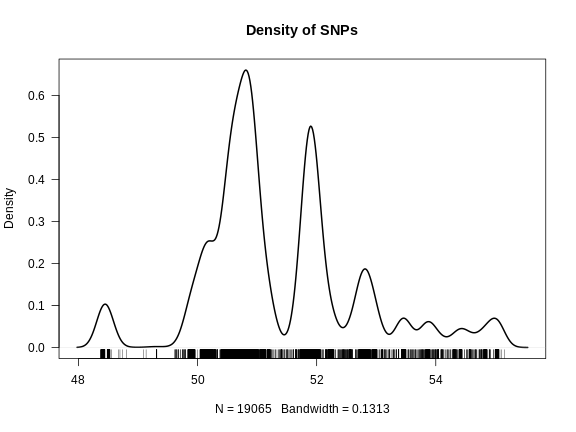
From the plot above, we can see that the density of SNPS between B6 and BTBR is not uniform. Most of the SNPs lie between 50 and 52 Mb, with less dense regions extending past 54 Mb.
The vcf object contains predicted SNP consequences in a
field called CSQ. The format of this field is challenging
to parse, so we will get it, search for missense and stop SNPs, and then
do some data-wrangling to may the output readable.
R
csq <- info(vcf_chr19)$CSQ
csq <- as.list(csq)

wh  <- grep('missense|stop', csq)
csq <- csq[wh]
rr  <- rowRanges(vcf_chr19)[wh]
Let’s see how many SNPs had missense or stop codon consequences.
R
length(csq)
OUTPUT
[1] 8There were only 8 SNPs out of 19,000 SNPs with missense or stop codon consequences. Next, let’s do the data wrangling to reformat the consequences of these SNPs.
R
csq <- lapply(csq, strsplit, split = "\\|")
csq <- lapply(csq, function(z) {
                     matrix(unlist(z), ncol = length(z[[1]]), byrow = TRUE)
                   })

for(i in seq_along(csq)) {

  csq[[i]] <- data.frame(snp_id = names(rr)[i],
                         csq[[i]])

} # for(i)

csq = do.call(rbind, csq)
Let’s look at the top of csq.
R
head(csq)
OUTPUT
           snp_id X1               X2       X3     X4                 X5
1 19:50141282_A/G  G   intron_variant MODIFIER Sorcs1 ENSMUSG00000043531
2 19:50141282_A/G  T   intron_variant MODIFIER Sorcs1 ENSMUSG00000043531
3 19:50141282_A/G  C   intron_variant MODIFIER Sorcs1 ENSMUSG00000043531
4 19:50141282_A/G  G missense_variant MODERATE Sorcs1 ENSMUSG00000043531
5 19:50141282_A/G  T missense_variant MODERATE Sorcs1 ENSMUSG00000043531
6 19:50141282_A/G  C missense_variant MODERATE Sorcs1 ENSMUSG00000043531
          X6                 X7             X8    X9   X10 X11 X12  X13  X14
1 Transcript ENSMUST00000072685 protein_coding       26/26
2 Transcript ENSMUST00000072685 protein_coding       26/26
3 Transcript ENSMUST00000072685 protein_coding       26/26
4 Transcript ENSMUST00000111756 protein_coding 27/27               3465 3448
5 Transcript ENSMUST00000111756 protein_coding 27/27               3465 3448
6 Transcript ENSMUST00000111756 protein_coding 27/27               3465 3448
   X15 X16     X17 X18 X19 X20 X21 X22 X23 X24               X25 X26 X27 X28
1                           -1     SNV MGI
2                           -1     SNV MGI
3                           -1     SNV MGI
4 1150 S/P Tct/Cct          -1     SNV MGI       tolerated(0.09)
5 1150 S/T Tct/Act          -1     SNV MGI       tolerated(0.26)
6 1150 S/A Tct/Gct          -1     SNV MGI     deleterious(0.03)
  X29
1
2
3
4
5
6
There are a lot of columns and we may not need all of them. Next, let’s reduce the number of columns to keep the ones that we need.
R
csq <- csq[,c(1:7,9,17,18,26)]
Next, we will subset the consequences to retain the unique rows and then retain rows which contain “missense” and “stop”.
R
csq <- distinct(csq) |>
         filter(str_detect(X2, "missense|stop"))
Let’s look at the top of csq now.
R
head(csq)
OUTPUT
           snp_id X1               X2       X3     X4                 X5
1 19:50141282_A/G  G missense_variant MODERATE Sorcs1 ENSMUSG00000043531
2 19:50141282_A/G  T missense_variant MODERATE Sorcs1 ENSMUSG00000043531
3 19:50141282_A/G  C missense_variant MODERATE Sorcs1 ENSMUSG00000043531
4 19:50141444_G/A  A missense_variant MODERATE Sorcs1 ENSMUSG00000043531
5 19:50141444_G/A  T missense_variant MODERATE Sorcs1 ENSMUSG00000043531
6 19:50141444_G/A  C missense_variant MODERATE Sorcs1 ENSMUSG00000043531
          X6             X8 X16     X17                              X25
1 Transcript protein_coding S/P Tct/Cct                  tolerated(0.09)
2 Transcript protein_coding S/T Tct/Act                  tolerated(0.26)
3 Transcript protein_coding S/A Tct/Gct                deleterious(0.03)
4 Transcript protein_coding S/F tCc/tTc deleterious_low_confidence(0.01)
5 Transcript protein_coding S/Y tCc/tAc deleterious_low_confidence(0.01)
6 Transcript protein_coding S/C tCc/tGc deleterious_low_confidence(0.01)
Column X4 contains gene names. Let’s get the unique gene
names.
R
csq |>
  distinct(X4)
OUTPUT
      X4
1 Sorcs1
2  Rbm20
There are only two genes in the QTL support interval which contain missense SNPs.
Challenge 4: Search Genes using Pubmed
- Go to Pubmed and search for papers involving the two genes and insulin or diabetes.
In this case, we used published SNPs data to identify two potential candidate genes. If we had not found publications that had already associated these genes with diabetes, these would be genes that you would follow up on in the lab.
Using Expression QTL Mapping
Another method of searching for candidate genes is to look for genes which have QTL peaks in the same location as the insulin QTL. Genes which have QTL that are co-located with insulin QTL will also be strongly correlated with insulin levels. These genes may be correlated with insulin because they control insulin levels, respond to insulin levels, or are correlated by chance. However, genes which have QTL within the insulin QTL support interval are reasonable candidate genes since we expect the genotype to influence expression levels.
Let’s perform QTL mapping on the genes within the chromosome 19
insulin QTL support interval. We can do this by passing in the
expression values as phenotypes into scan1.
R
eqtl_chr19 <- scan1(genoprobs = probs[,chr],
                    pheno     = expr_chr19,
                    kinship   = kinship_loco[[chr]],
                    addcovar  = addcovar)
Let’s look at the top of the results.
R
head(eqtl_chr19[,1:6])
OUTPUT
           498370 500695 501344 504488 505754 506116
rs4232073    2.38   2.02  0.766  0.279  0.918 0.1567
rs13483548   2.34   2.01  0.778  0.279  0.919 0.1567
rs13483549   2.33   2.00  0.784  0.278  0.913 0.1489
rs13483550   2.23   1.72  0.865  0.245  0.765 0.0618
rs13483554   1.94   1.69  0.886  0.249  0.819 0.1127
rs13483555   2.08   1.62  0.862  0.255  0.867 0.1289
The eQTL results have one row for each marker and one column for each gene. Each column represents the LOD plot for one gene. Let’s plot the genome scan for one gene.
R
gene_id <- '10002678668'
symbol  <- annot_chr19$gene_name[annot_chr19$a_gene_id == gene_id]

plot_scan1(x   = eqtl_chr19,
           map = cross$pmap,
           lodcolumn = gene_id,
           main      = symbol)
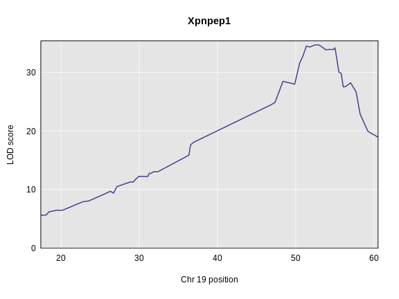
This gene seems to have a QTL on chromosome 19 near 52 Mb with a LOD of 34. The insulin QTL is closer to 55 Mb, so this may be a good candidate gene.
We can harvest the significant QTL peaks on chromosome 19 using
find_peaks. We will use the default threshold of LOD =
3.
R
eqtl_chr19_peaks <- find_peaks(eqtl_chr19, map = cross$pmap) |>
                      arrange(pos)
eqtl_chr19_peaks
OUTPUT
  lodindex   lodcolumn chr  pos   lod
1       21 10004035475  19 47.4  4.66
2       17 10002936879  19 51.4  7.66
3       16 10002928587  19 51.8  7.12
4       11 10002678668  19 52.4 34.67
5        1      498370  19 53.0 12.39
6       14 10002910800  19 54.8  4.23
We can see that there are 6 significant QTL on chromosome 19. All of these genes are within the support interval of the insulin QTL.
Let’s filter the eQTL genes and add in gene annotation for them.
R
eqtl_chr19_peaks <- eqtl_chr19_peaks |>
                     filter(pos > peaks_chr19$ci_lo & pos < peaks_chr19$ci_hi) |>
                     left_join(annot, by = c('lodcolumn' = 'a_gene_id'))
eqtl_chr19_peaks
OUTPUT
  lodindex   lodcolumn chr.x  pos   lod chr.y start  end  width strand
1       17 10002936879    19 51.4  7.66    19  53.7 53.9 189775      +
2       16 10002928587    19 51.8  7.12    19  50.1 50.7 535348      -
3       11 10002678668    19 52.4 34.67    19  52.9 53.0 108289      -
4        1      498370    19 53.0 12.39    19  53.4 53.4  11189      -
5       14 10002910800    19 54.8  4.23    19  52.3 52.3   1180      +
             gene_id gene_name   gene_biotype
1 ENSMUSG00000043639     Rbm20 protein_coding
2 ENSMUSG00000043531    Sorcs1 protein_coding
3 ENSMUSG00000025027   Xpnpep1 protein_coding
4 ENSMUSG00000025024    Smndc1 protein_coding
5 ENSMUSG00000035804      Ins1 protein_coding
                                                                                description
1                          RNA binding motif protein 20 [Source:MGI Symbol;Acc:MGI:1920963]
2   sortilin-related VPS10 domain containing receptor 1 [Source:MGI Symbol;Acc:MGI:1929666]
3 X-prolyl aminopeptidase (aminopeptidase P) 1, soluble [Source:MGI Symbol;Acc:MGI:2180003]
4             survival motor neuron domain containing 1 [Source:MGI Symbol;Acc:MGI:1923729]
5                                               insulin I [Source:MGI Symbol;Acc:MGI:96572]
        gene_id_version  symbol entrezid
1 ENSMUSG00000043639.16   Rbm20       NA
2 ENSMUSG00000043531.17  Sorcs1       NA
3 ENSMUSG00000025027.19 Xpnpep1       NA
4  ENSMUSG00000025024.8  Smndc1       NA
5  ENSMUSG00000035804.6    Ins1       NA
Let’s plot the insulin QTL again to remind ourselves what the peak on chromosome 19 look like. We will also plot the genome scan for one of the genes on chromosome 19.
R
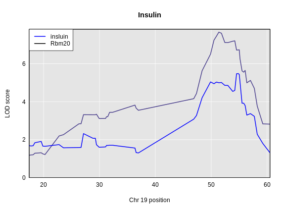
gene_id <- "10002936879"
symbol  <- annot_chr19$gene_name[annot_chr19$a_gene_id == gene_id]

plot_scan1(x    = eqtl_chr19,
           map  = cross$pmap,
           lodcolumn = gene_id,
           main = "Insulin")
plot_scan1(x    = lod_add_loco,
           map  = cross$pmap,
           chr  = '19',
           col  = 'blue',
           add  = TRUE)
legend("topleft", legend = c("insluin", symbol),
       col = c('blue', 'black'), lwd = 2)
Why would we prioritize genes with an eQTL in the same location as an insulin QTL? If a gene has an eQTL in the same location, there are genetic variants which influence it’s expression at that location. These variants may be distinct from the ones which influence the phenotype or they may influence gene expression which then influences the phenotype. We call this causal relationship of a SNP changing expression, which then changes the phenotype, “mediation”.
Mediation Analysis
If a gene is correlated with insulin levels and if it has an eQTL in the same location as insulin, then we could add it into the insulin QTL model and see if it reduces the LOD on chromosome 19.
R
stopifnot(rownames(addcovar) == rownames(expr_chr19))
addcovar_chr19 <- cbind(addcovar, expr_chr19[,"10002936879"])

lod_med <- scan1(genoprobs = probs[,chr],
                 pheno     = insulin,
                 kinship   = kinship_loco[[chr]],
                 addcovar  = addcovar_chr19)
Next, we will plot the original insulin genome scan and overlay the
genome scan with gene 10002936879 in the model.
R
gene_id <- "10002936879"
symbol  <- annot_chr19$gene_name[annot_chr19$a_gene_id == gene_id]

plot_scan1(x    = lod_add_loco,
           map  = cross$pmap,
           chr  = '19',
           main = paste("Insulin with/without", symbol))
plot_scan1(x    = lod_med,
           map  = cross$pmap,
           chr  = '19',
           col  = "blue",
           add  = TRUE)
legend("topleft", legend = c("insluin", "mediation"),
       col = c('black', 'blue'), lwd = 2)
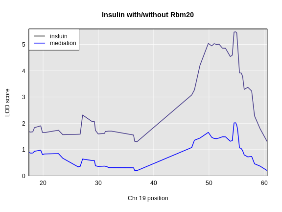
The LOD dropped from 5.477 to 2.02. This is a difference of 3.456.
It would be slow to run a genome scan for each gene on chromosome 19
and look at the LOD drop. Also, we don’t really need the LOD drop across
the entire chromosome. We only need the LOD drop at the location of the
peak LOD. To do this, we can use the fit1 function to get
the LOD at the marker with the highest LOD in the insulin genome
scan.
R
# Get the probs at the maximum insulin QTL on Chr 19.
pr_chr19 = pull_genoprobpos(genoprobs = probs,
                            map       = cross$pmap,
                            chr       = chr,
                            pos       = peaks_chr19$pos)

# Create data sructure for results.
lod_drop = data.frame(a_gene_id = colnames(expr_chr19),
                      lod       = 0)

for(i in 1:ncol(expr_chr19)) {

  # Make new covariates.
  curr_covar = cbind(addcovar, expr_chr19[,i])

  # Fit the insulin QTL model with the gene as a covariate.
  mod = fit1(genoprobs = pr_chr19,
             pheno     = insulin,
             kinship   = kinship_loco[[chr]],
             addcovar  = curr_covar)

  # Save the LOD.
  lod_drop$lod[i] = mod$lod

} # for(i)

# Subtract the insulin LOD from the mediation LODs.
lod_drop$lod_drop = lod_drop$lod - peaks_chr19$lod
R
lod_drop <- left_join(lod_drop, annot_chr19, by = 'a_gene_id')

plot(lod_drop$start, lod_drop$lod_drop, col = NA,
     main = "Mediation Analysis on Chr 19",
     xlab = "Posiiton (Mb)", ylab = "LOD Drop")
text(lod_drop$start, lod_drop$lod_drop, labels = lod_drop$gene_name)
abline(v = peaks_chr19$pos, col = 2)
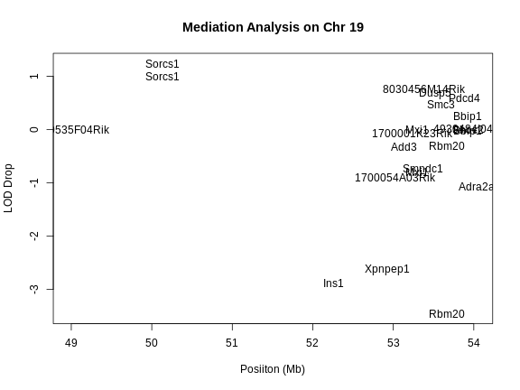
In the plot above, we plotted the position of each gene versus the decrease in the LOD score (i.e. LOD drop). Genes with the lowest LOD drop are the best candidate genes based on mediation analysis.
Let’s look at the annotation for the genes with LOD drop less than -2.
R
lod_drop |>
  filter(lod_drop < -2) |>
  select(gene_id, symbol, chr, start, end, lod, lod_drop, description)
OUTPUT
             gene_id  symbol chr start  end  lod lod_drop
1 ENSMUSG00000025027 Xpnpep1  19  52.9 53.0 2.85    -2.63
2 ENSMUSG00000035804    Ins1  19  52.3 52.3 2.60    -2.88
3 ENSMUSG00000043639   Rbm20  19  53.7 53.9 2.02    -3.46
                                                                                description
1 X-prolyl aminopeptidase (aminopeptidase P) 1, soluble [Source:MGI Symbol;Acc:MGI:2180003]
2                                               insulin I [Source:MGI Symbol;Acc:MGI:96572]
3                          RNA binding motif protein 20 [Source:MGI Symbol;Acc:MGI:1920963]
Do you see any good candidate genes which might regulate insulin?
Summary
In this episode, we learned how to identify candidate genes under a QTL peak. In a perfect world, there would be exactly one gene implicated by these analyses. In most cases, you will have a set of candidate genes and you will need to study each gene and prioritize some for laboratory follow-up.
There are two ways of searching for candidate genes: using SNPs in the QTL interval, and looking for genes with eQTL which are co-located with the phenotype QTL. We learned how to query a VCF file and how to perform mediation analysis. After this step, you will have a set of genes which you can test for association with your phenotype.
- There will be many genes under a QTL peak.
- You can search for genes with SNPs that produce coding changes by querying a VCF file.
- You can search for genes with expression changes that may influence your phenotype by performing mediation analysis with expression data from the same mice.