Summary and Setup
Quantitative trait mapping is used in biomedical, agricultural, and evolutionary studies to find causal genes for quantitative traits, to aid crop and breed selection in agriculture, and to shed light on natural selection. Examples of quantitative traits include cholesterol level, plant yield, or egg size, all of which are continuous variables. The goal of quantitative trait locus (QTL) analysis is to identify genomic regions linked to a phenotype, to map these regions precisely, and to define the effects, number, and interactions of QTL.
QTL analysis can be performed in natural populations or in experimental crosses, and can be studied in humans and non-human species. Human studies, however, are very expensive, lack environmental control, and can be confounded by population structure such that associations between genotype and phenotype are not necessarily causal.
QTL analysis in experimental crosses requires two or more strains that differ genetically with regard to a phenotype of interest. Genetic markers, such as SNPs or microsatellites, distinguish between parental strains in the experimental cross. Markers that are genetically linked to a phenotype will segregate more often with phenotype values (high or low values, for example), while unlinked markers will not be significantly associated with the phenotype. The markers themselves might be associated with the phenotype but are not causal. Rather, markers may be associated with the phenotype through linkage to nearby QTL. They serve as signposts indicating the neighborhood of a QTL that influences a phenotype. Covariates such as sex or diet can also influence the phenotype.
R/qtl2 (aka qtl2) is a reimplementation of the QTL analysis software R/qtl to better handle high-dimensional data and complex cross designs such as the Diversity Outbred. Typically R/qtl2 will be employed in “batch” (for example, on a cluster) rather than interactively.
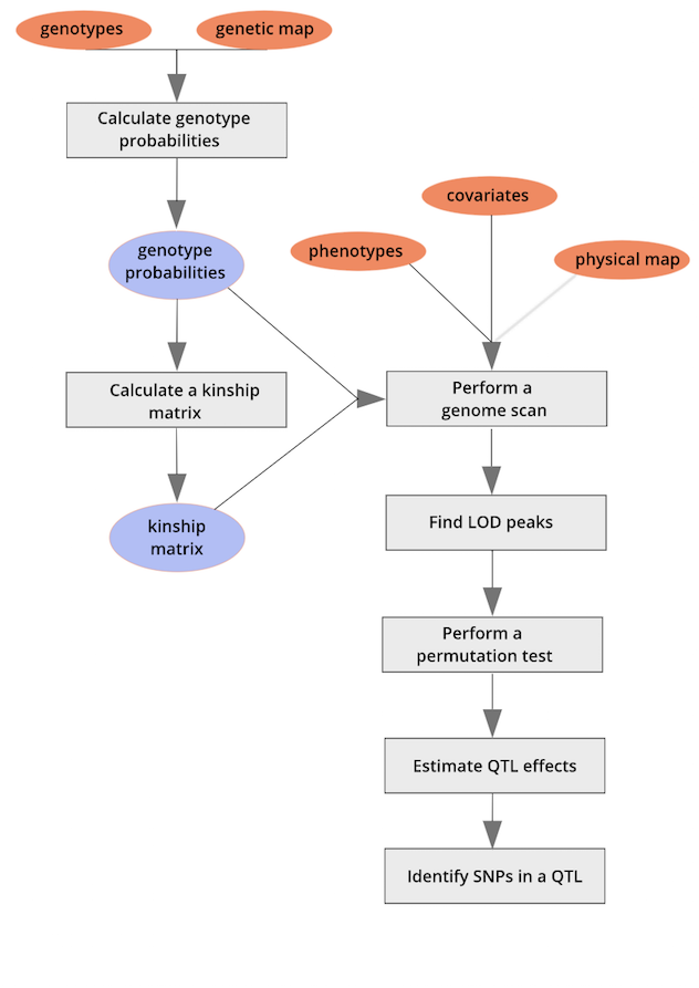
This lesson will focus on the R/qtl2 package in R. A workflow for quantitative trait mapping with R/qtl2 is shown here.

To cite R/qtl in publications: Broman KW, Wu H, Sen S, Churchill GA (2003) R/qtl: QTL mapping in experimental crosses. Bioinformatics 19:889-89
Software Setup
R is a programming language that is especially powerful for data exploration, visualization, and statistical analysis. To interact with R, we use RStudio.
Install the latest version of R from CRAN.
Install the latest version of RStudio. Choose the free RStudio Desktop version for Windows, Mac, or Linux.
Start RStudio.
-
Install packages.
- The qtl2 package contains code for haplotype reconstruction, QTL mapping and plotting.
- The qtl2convert package contains code for converting data objects from one format to another.
- Install qtl2 by copying and pasting the following code in the R console.
R
install.packages(c("tidyverse", "ggbeeswarm", "qtl2", "qtl2convert"))
Once the installation is complete, load the libraries to make sure that they installed correctly.
R
library(tidyverse)
library(ggbeeswarm)
library(qtl2)
library(qtl2convert)
If the libraries don’t load and you received errors during the installation, please contact the workshop instructors before the workshop to help you.
Project organization
- Create a new project in your Desktop called
qtl_mapping.
- Click the
Filemenu button, thenNew Project. - Click
New Directory. - Click
New Project. - Type
qtl_mappingas the directory name. Browse to your Desktop to create the project there. - Click the
Create Projectbutton.
- Use the
Filestab to create adatafolder to hold the data, ascriptsfolder to house your scripts, and aresultsfolder to hold results. Alternatively, you can use the R console to run the following commands for step 2 only. You still need to create a project with step 1.
R
dir.create("./data")
dir.create("./scripts")
dir.create("./results")
Data Sets
For this course, we will have several data files which you will need
to download to the data directory in the project folder on
your Desktop. Copy, paste, and run the following code in the RStudio
console.
The first file contains the data that we will use for QTL mapping in an F2 population. Download it using the code below.
R
download.file(url      = "https://thejacksonlaboratory.box.com/shared/static/svw7ivp5hhmd7vb8fy26tc53h7r85wez.zip",
              destfile = "data/attie_b6btbr_grcm39.zip",
              mode     = "wb")

unzip(zipfile = "data/attie_b6btbr_grcm39.zip",
      exdir   = "./data/")
The second file contains the Diversity Outbred mapping data.
R
download.file(url      = "https://thejacksonlaboratory.box.com/shared/static/wspizp2jgrtngvvw5ixredpu7627mh5w.rdata",
              destfile = "data/qtl2_demo_grcm39.Rdata",
              mode     = "wb")
Next, download the MUGA marker positions from Karl Broman’s Github page.
R
download.file(url      = "https://raw.githubusercontent.com/kbroman/MUGAarrays/main/UWisc/muga_uwisc_v4.csv",
              destfile = "data/muga_uwisc_v4.csv",
              mode     = "wb")
Next, we need a database of the DO founder SNPs and gene positions. This file is 10 GB, so it will take a while to download.
R
download.file(url      = "https://figshare.com/ndownloader/files/40157572",
              destfile = "data/fv.2021.snps.db3",
              mode     = "wb")
If you get an error message downloading this file from figshare, use
a web browser to download from the URL. Go to https://figshare.com/ndownloader/files/40157572
to start the download. Then move the file from wherever your downloads
go (e.g. Downloads) to the data
directory in the qtl_mapping project. You can use a
graphical user interface (e.g. Windows File Explorer, Mac
Finder) to move the file.
Development of this lesson was funded by NIH award GM070683 to Dr. Gary Churchill at The Jackson Laboratory.
