Calculating Genotype Probabilities
Last updated on 2025-09-30 | Edit this page
Overview
Questions
- How do I calculate QTL at positions between genotyped markers?
- How do I calculate QTL genotype probabilities?
- How do I calculate allele probabilities?
- How can I speed up calculations if I have a large data set?
Objectives
- To explain why the first step in QTL analysis is to calculate genotype probabilities.
- To calculate genotype probabilities.
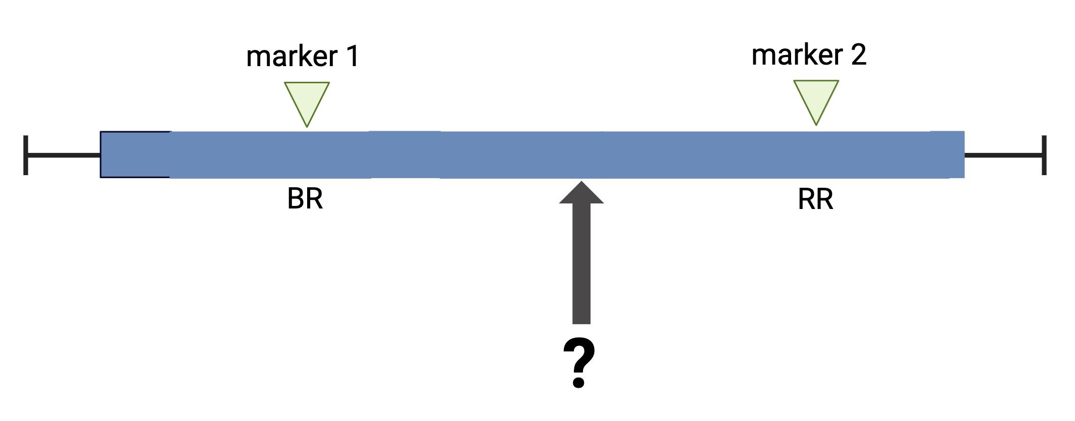
The first task in QTL analysis is to calculate conditional genotype probabilities, given the observed marker data, at each putative QTL position. For example, the first step would be to determine the probabilities for genotypes BR and RR at the locus indicated below.

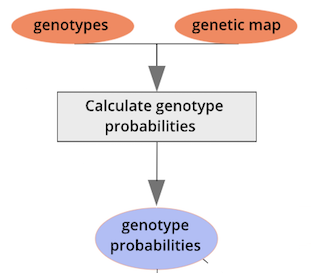
The calc_genoprob() function calculates QTL genotype
probabilities conditional on the available marker data. These are needed
for most of the QTL mapping functions. The result is returned as a list
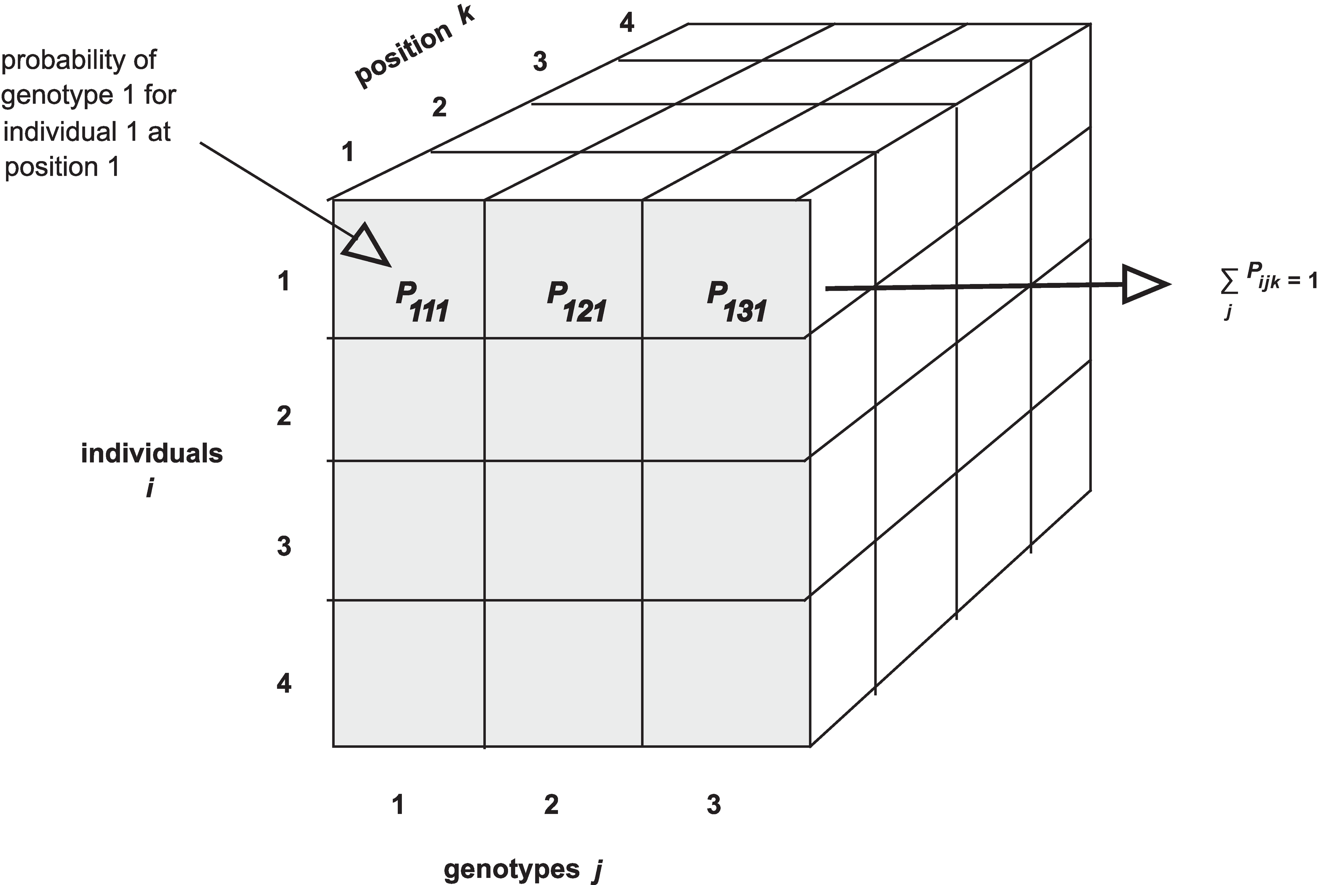
of three-dimensional arrays (one per chromosome). Each 3d array of
probabilities is arranged as individuals \(\times\) genotypes \(\times\) positions.

 Notice that arrays in R require data to be all of the same type - all
numeric, all character, all Boolean, etc. If you are familiar with data
frames in R you know that you can mix different kinds of data in that
structure. The first column might contain numeric data, the second
column character data, the third Boolean (True / False), and so on.
Arrays won’t accept mixed data types though.
We’ll use the Attie
BL6/BTBR dataset from Tian et
al (an intercross) as an example. In this study, circulating insulin
levels were measured in an F2 cross between mouse strains C57BL/6J and
BTBTR T+
First, we will load in the qtl2 library, which provides the functions that we will use for QTL analysis.
R
library(qtl2)
The function read_cross2() has a single argument: the
name (with path) of the control file, or alternatively a zip file
containing all the required data. We read in the data with a JSON
control file like this:
R
cross <- read_cross2(file = 'data/attie_control.json')
To load your own data from your machine, you would use the file path
to your data files. For example, if the file path to your data files is
/Users/myUserName/qtlProject/data, the command to load your
data would look like this:
R
myQTLdata <- read_cross2(file = "/Users/myUserName/qtlProject/data/myqtldata.json" )
The JSON file contains all control information for your data, including names of data files, cross type, column specifications for sex and cross information, and more. This can also be in YAML format. Alternatively, all data files can be zipped together for loading.
R
myQTLdata <- read_cross2(file = "/Users/myUserName/qtlProject/data/myqtldata.zip" )
Back to the BTBR data. Now look at a summary of the cross data and the names of each variable within the data.
R
summary(cross)
OUTPUT
Object of class cross2 (crosstype "f2")

Total individuals             490
No. genotyped individuals     490
No. phenotyped individuals    490
No. with both geno & pheno    490

No. phenotypes                  3
No. covariates                  8
No. phenotype covariates        0

No. chromosomes                20
Total markers                2057

No. markers by chr:
  1   2   3   4   5   6   7   8   9  10  11  12  13  14  15  16  17  18  19   X
156 135 157 126 125 102 109  91  93 123 124 116 116  91 102  66  60  95  50  20
R
names(cross)
OUTPUT
 [1] "crosstype"  "geno"       "gmap"       "pmap"       "pheno"
 [6] "covar"      "is_x_chr"   "is_female"  "cross_info" "alleles"
Challenge 1
1). How many mice are in this study?
2). How many phenotypes are there?
3). How many markers?
4). How many markers are on chr 11?
The output of summary(cross) provides this
information.
1). There are 490 individuals in the cross.
2). 3 phenotypes
3). 2,057 markers
4). 124 markers on chromosome 11
Have a look at the markers listed in the genetic map,
gmap. Markers are listed by chromosome and described by cM
position. View only the markers on the first two chromosomes.
R
head(cross$gmap, n=1)
OUTPUT
$`1`
rs13475697  rs3681603 rs13475703 rs13475710  rs6367205 rs13475716 rs13475717
 0.1881141  0.1920975  0.4167755  0.6488793  0.6555814  0.6638576  0.6676198
rs13475719 rs13459050  rs3680898 rs13475727 rs13475728 rs13475729 rs13475731
 0.6711377  0.6749344  0.6775292  1.8149573  1.9596637  2.3456569  2.7186389
rs13475737 rs13475744  rs6397513 rs13475747 rs13475748 rs13475749 rs13475750
 3.1059517  3.8222865  4.3094607  4.3120150  4.5098582  4.8154609  4.8853505
rs13475751 rs13475752 rs13475762 rs13475764 rs13475765 rs13475768 rs13475769
 4.8869793  4.8902179  7.2954871  8.2102887  8.3708197  8.7178703  8.8859153
rs13475771  rs6384194 rs13475790  rs3676270 rs13475794 rs13475801  rs4222269
 9.1374722  9.9295192  9.9970634 10.1508878 10.3962716 11.5981956 11.9606369
 rs6387241 rs13475822 rs13475824 rs13475826 rs13475827 rs13475834 rs13475880
16.8770742 16.9815396 17.4434784 18.0866148 18.6276972 19.2288050 27.4056813
rs13475883  rs6239834  rs3162895  rs6212146  rs3022802 rs13475899 rs13475900
28.4641674 30.8427150 31.1526514 31.2751278 31.3428706 31.8493556 31.8518088
rs13475906  rs3022803 rs13475907 rs13475909 rs13475912  rs6209698 rs13475929
32.2967145 32.3074644 32.3683291 32.8001894 33.6026526 36.5341646 37.6881435
rs13475931 rs13475933 rs13475934  rs4222476 rs13475939  rs8253473 rs13475941
37.7429827 38.0416271 38.0430095 38.9647582 39.4116688 39.4192277 39.4871064
rs13475944 rs13475947 rs13475948 rs13475950 rs13475951 rs13475954 rs13475955
39.7672829 40.2599440 40.3380113 40.3417592 40.3439501 41.1407252 41.2887176
rs13475963 rs13475966 rs13475967 rs13475970 rs13475960  rs6250696 rs13475973
42.4744416 42.5667702 42.9736574 43.1427994 43.5985261 43.5992946 43.6014053
 rs3691187 rs13475988 rs13475991 rs13476023 rs13476024  rs3684654  rs6274257
44.6237384 45.7855528 46.0180221 47.8579278 47.8600317 48.2423958 48.9612178
rs13476045 rs13476049  rs6319405 rs13476050 rs13476051 rs13476054 rs13476057
49.2018340 49.3701384 49.4261039 49.4275718 49.4323558 49.4972616 49.5031830
rs13476059 rs13476060 rs13476062 rs13476066 rs13476067  rs6259837 rs13476080
49.5084008 49.5113545 49.6085043 49.6644819 50.1779477 50.8256056 51.0328603
 rs6302966 rs13476085 rs13476089  rs3717360 rs13476090  rs6248251 rs13476091
51.3659553 51.6974451 52.3869798 52.3903517 52.3936241 52.4228715 52.5787388
 rs3088725  rs3022832  rs4222577 rs13476100  rs6263067  rs8256168  rs6327099
53.4044231 53.4129004 53.4189013 54.3267003 54.4193890 55.1459517 55.3274320
rs13476111 rs13476119  rs8236484  rs8270838  rs8236489 rs13476129 rs13476134
55.9050491 56.8936305 56.9852502 57.1870637 58.0248893 58.7605079 59.5401544
rs13476135 rs13476137 rs13476138 rs13476140 rs13476148  rs6202860 rs13476158
59.5426193 59.6023794 60.3355828 60.3439598 61.1791787 61.9905512 61.9930265
rs13476163 rs13476177 rs13476178 rs13476183 rs13476184  rs6194543 rs13476196
62.0039607 62.6243588 62.6269118 63.8101331 64.0856907 66.4047817 66.7425394
rs13476201  rs3685700  rs3022846 rs13476210 rs13476214 rs13459163  rs4222816
67.2638714 68.7230251 68.7246243 69.1209547 70.1550813 75.5548371 75.5593190
 rs4222820  rs3090340  rs8245949 rs13476242 rs13476251 rs13476254  rs6383012
75.5593202 75.5637846 76.7508053 79.0157673 79.7644000 79.8248805 85.3173344
rs13476279  rs6348421 rs13476290 rs13476300 rs13476302 rs13476304  rs3669814
86.7653503 88.2128991 89.0565541 94.6215368 94.8227821 94.8269227 95.5413280
rs13501301 rs13476316
96.0784002 96.9960494
Next we use calc_genoprob() to calculate the QTL
genotype probabilities.
R
probs <- calc_genoprob(cross      = cross,
                       map        = cross$gmap,
                       error_prob = 0.002)
The argument error_prob supplies an assumed genotyping
error probability of 0.002. If a value for error_prob is
not supplied, the default probability is 0.0001.
Recall that the result of calc_genoprob,
probs, is a list of three-dimensional arrays (one per
chromosome).
R
names(probs)
OUTPUT
 [1] "1"  "2"  "3"  "4"  "5"  "6"  "7"  "8"  "9"  "10" "11" "12" "13" "14" "15"
[16] "16" "17" "18" "19" "X"
Each three-dimensional array of probabilities is arranged as individuals \(\times\) genotypes \(\times\) positions. Have a look at the names of each of the three dimensions for chromosome 19.
R
head(dimnames(probs$`19`)[[1]])
OUTPUT
[1] "Mouse3051" "Mouse3551" "Mouse3430" "Mouse3476" "Mouse3414" "Mouse3145"R
dimnames(probs$`19`)[2]
OUTPUT
[[1]]
[1] "BB" "BR" "RR"
R
dimnames(probs$`19`)[3]
OUTPUT
[[1]]
 [1] "rs4232073"  "rs13483548" "rs13483549" "rs13483550" "rs13483554"
 [6] "rs13483555" "rs3090321"  "rs3090137"  "rs6309315"  "rs13483577"
[11] "rs3090325"  "rs13483579" "rs13483584" "rs13483586" "rs13483587"
[16] "rs13483589" "rs13483592" "rs13483593" "rs6344448"  "rs13483594"
[21] "rs13483595" "rs3705022"  "rs13483609" "rs13483612" "rs13483648"
[26] "rs13483650" "rs13483654" "rs13483658" "rs13483660" "rs13483664"
[31] "rs13483666" "rs13483667" "rs13483670" "rs8275553"  "rs8275912"
[36] "rs13483677" "rs13483679" "rs13483680" "rs13483681" "rs3660143"
[41] "rs13483682" "rs13483683" "rs13483685" "rs13483686" "rs6355398"
[46] "rs4222106"  "rs13483690" "rs13483693" "rs13483695" "rs13483699"
View the first three rows of genotype probabilities for the first genotyped marker on chromosome 19.
R
(probs$`19`)[1:5, , "rs4232073"]
OUTPUT
                    BB           BR           RR
Mouse3051 1.317728e-11 1.235895e-07 9.999999e-01
Mouse3551 9.999840e-01 1.595361e-05 5.027172e-08
Mouse3430 1.317728e-11 1.235895e-07 9.999999e-01
Mouse3476 9.999999e-01 1.235895e-07 1.317728e-11
Mouse3414 6.179474e-08 9.999999e-01 6.179474e-08
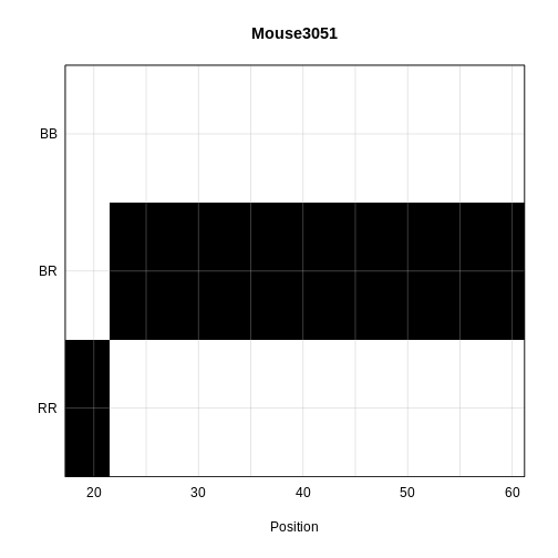
We can also view the genotype probabilities using plot_genoprob. The arguments to this function specify:
-
probs: the genotype probabilities, -
map: the marker map, -
ind: the index of the individual to plot, -
chr: the index of the chromosome to plot.
R
plot_genoprob(probs = probs,
              map   = cross$pmap,
              ind   = 1,
              chr   = 19,
              main  = rownames(probs[['19']])[1])

The coordinates along chromosome 19 are shown on the horizontal axis and the three genotypes are shown on the vertical axis. Higher genotype probabilities are plotted in darker shades. This mouse has a RR genotype on the proximal end of the chromosome and transitions to BR.

Challenge 2
1). Load a second dataset from the qtl2data repository. Locate
the BXD
directory and load the data directly from the web using this code
given at the bottom of the ReadMe.md file.
file <- paste0("https://raw.githubusercontent.com/rqtl/", "qtl2data/main/BXD/bxd.zip").
bxd <- read_cross2(file)
2). How many individuals were in the study? How many phenotypes? How many markers?
3). Calculate genotype probabilities and save the results to an
object called bxdpr. View the genotypes for the first three
markers on chromosome 1 for the first five individuals.
1).
file <- paste0("https://raw.githubusercontent.com/rqtl/", "qtl2data/main/BXD/bxd.zip").bxd <- read_cross2(file)
2). summary(bxd) gives 198 individuals, 5,806 phenotypes
and 7,320 markers.
3). bxdpr <- calc_genoprob(cross = bxd, map = bxd$gmap)
followed by(bxdpr$1)[1:5, , 1:3]
Challenge 3
Plot the genotype probabilities for individual number 3 for chromosome 1.
plot_genoprob(probs = bxdpr, map = bxd$pmap, ind = 3, chr = 1, main = rownames(bxdpr[['1']])[3])
Parallel calculations (optional) To speed up the
calculations with large datasets on a multi-core machine, you can use
the argument cores. With cores=0, the number
of available cores will be detected via
parallel::detectCores(). Otherwise, specify the number of
cores as a positive integer.
R
probs <- calc_genoprob(cross = iron,
                         map = map,
                  error_prob = 0.002,
                       cores = 4)
Allele probabilities (optional) The genome scan
functions use genotype probabilities as well as a matrix of phenotypes.
If you wished to perform a genome scan via an additive allele model, you
would first convert the genotype probabilities to allele probabilities,
using the function genoprob_to_alleleprob().
R
apr <- genoprob_to_alleleprob(probs = probs)
- The first step in QTL analysis is to calculate genotype probabilities.
- Calculate genotype probabilities between genotyped markers with
calc_genoprob().
