Calculating A Kinship Matrix
Last updated on 2025-09-30 | Edit this page
Overview
Questions
- Why would I calculate kinship between individuals?
- How do I calculate kinship between individuals?
- What does a kinship matrix look like?
Objectives
- Explain why and when kinship calculation matters in mapping.
- Create a kinship matrix for individuals.
Population structure and kinship are common confounding factors in genome-wide association studies (GWAS), case-control studies, and other study types in genetics. They create false positive associations between genotype and phenotype at genetic markers that differ in genotype frequencies between subpopulations due to genetic relatedness between samples. Simple association tests assume statistical independence between individuals. Population structure and kinship confound associations when phenotype covariance between individuals results from genetic similarity. Accounting for relatedness between individuals helps to distinguish true associations from false positives generated by population structure or kinship.
As an example see the table below for phenotype and genotype frequencies between two subpopulations in a case-control study.
| subpop1 | subpop2 | overall pop | |
|---|---|---|---|
| frequency | 0.5 | 0.5 | 1 |
| probability of AA genotype | 0.1 | 0.9 | 0.5 |
| probability of disease | 0.9 | 0.1 | 0.5 |
| probability of disease & AA | 0.09 | 0.09 | 0.09 |
The full population consists of two equally represented subpopulations. In the overall population, the probability of the AA genotype is 0.5, and the probability of disease is also 0.5. The joint probability of both disease and AA genotype in the population (0.09) is less than either the probability of disease (0.5) or the probability of the AA genotype (0.5) alone, and is considerably less than the joint probability of 0.25 that would be calculated if subpopulations weren’t taken into account. In a case-control study that fails to recognize subpopulations, most of the cases will come from subpopulation 1 since this subpopulation has a disease probability of 0.9. However, this subpopulation also has a low probability of the AA genotype. So a false association between AA genotype and disease would occur because only overall population probabilities would be considered.
Kinship Calculation
In the B6/BTBR cross, we have three possible genotypes: BB, BR, and RR. Suppose that we look at the genotypes of two mice and estimate their kinship. To do this, we select the first allele from mouse 1 and get the probability of picking the same allele from mouse 2. Then we do the same procedure with the second allele and take the mean. This calculates the mean allele-sharing at that marker. We do this for all markers and take the overall mean.
Let’s look at an example. In the table below, we have listed four markers and their genotypes in mouse 1 (M1) and mouse 2 (M2). At each marker, we applied the procedure above and recorded the allele-sharing. Then we took the mean and found that these two mice have a kinship value of 0.5.
| marker | M1 | M2 | allele-sharing |
|---|---|---|---|
| 1 | BB | BB | 1.0 |
| 2 | BB | BR | 0.5 |
| 3 | BB | RR | 0.0 |
| 4 | BR | BR | 0.5 |
| — | – | – | — |
| All | – | – | 0.5 |
Challenge 1: Calculate the kinship of the following two sets of mice.
| marker | M1 | M2 |
|---|---|---|
| 1 | BB | RR |
| 2 | BB | RR |
| 3 | BB | RR |
| 4 | BB | BR |
| marker | M1 | M2 |
|---|---|---|
| 1 | BB | BR |
| 2 | BB | BR |
| 3 | RR | RR |
| 4 | RR | RR |
| marker | M1 | M2 | allele-sharing |
|---|---|---|---|
| 1 | BB | RR | 0.0 |
| 2 | BB | RR | 0.0 |
| 3 | BB | RR | 0.0 |
| 4 | BB | BR | 0.5 |
| — | – | – | — |
| All | – | – | 0.125 |
| marker | M1 | M2 | allele-sharing |
|---|---|---|---|
| 1 | BB | BR | 0.5 |
| 2 | BB | BR | 0.5 |
| 3 | RR | RR | 1.0 |
| 4 | RR | RR | 1.0 |
| — | – | – | — |
| All | – | – | 0.75 |
Linear mixed models (LMMs) consider genome-wide similarity between
all pairs of individuals to account for population structure, known
kinship and unknown relatedness. They model the covariance between
individuals. Linear mixed models in association mapping studies can
successfully correct for genetic relatedness between individuals in a
population by incorporating kinship into the model. To perform a genome
scan by a linear mixed model, accounting for the relationships among
individuals (in other words, including a random polygenic effect),
you’ll need to calculate a kinship matrix for the individuals. This is
accomplished with the calc_kinship() function. It takes the
genotype probabilities as input.
R
kinship <- calc_kinship(probs = probs)
Take a look at the kinship values calculated for the first 5 individuals.
R
kinship[1:5, 1:5]
OUTPUT
          Mouse3051 Mouse3551 Mouse3430 Mouse3476 Mouse3414
Mouse3051     0.737     0.501     0.535     0.520     0.510
Mouse3551     0.501     0.758     0.515     0.512     0.499
Mouse3430     0.535     0.515     0.749     0.458     0.493
Mouse3476     0.520     0.512     0.458     0.749     0.434
Mouse3414     0.510     0.499     0.493     0.434     0.696
We can also look at the first 50 mice in the kinship matrix.
R
n_samples <- 50
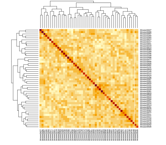
heatmap(kinship[1:n_samples, 1:n_samples], symm = TRUE)

The mice are listed in the same order on both sides of the matrix. The comb-like structures are called “dendrograms” and they indicate how the mice are clustered together. Each cell represents the degree of allele sharing between mice. Red colors indicate higher kinship and yellow colors indicate lower kinship. Each mouse is closely related to itself, so the cells along the diagonal tend to be darker than the other cells. You can see some evidence of related mice, possibly siblings, in the orange-shaded blocks along the diagonal.
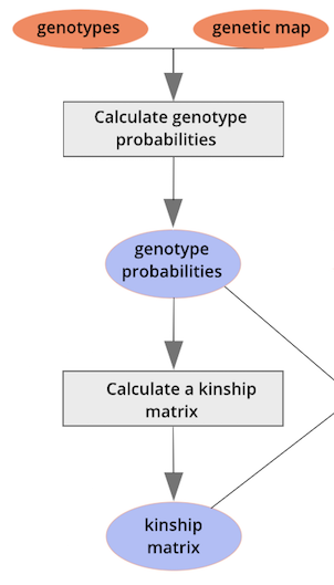
 {alt=“Part
of the mapping workflow starting with genotypes and a genetic map used
to calculate genotype probabilities, which are then used to calculate
kinship between individuals in the data.} By default, the genotype
probabilities are converted to allele probabilities, and the kinship
matrix is calculated as the proportion of shared alleles. Also by
default we omit the X chromosome and only use the autosomes. To include
the X chromosome, use
 omit_x=FALSE.
On a multi-core machine, you can get some speed-up via the
cores argument, as with calc_genoprob().
R
kinship <- calc_kinship(probs = probs,
                        cores = 4)
Challenge 2: What is a Kinship Matrix?
Think about what a kinship matrix is and what it represents. Share your understanding with a neighbor. Write your explanation in the collaborative document or in your own personal notes.
Challenge 3: Mean Value in Kinship Matrix
What is the mean kinship value of all mice? Can you explain why the value is the number that you get? Think about the three possible genotypes in the cross and how they compare to each other.
R
mean(kinship)
OUTPUT
[1] 0.501The mean kinship between the mice in the cross is 0.5. All of the mice were derived from F1 parents created from two inbred strains. The kinship calculation compares the number of identical alleles between mice at each marker. On average, each mouse carries 50% B alleles and 50% R alleles. So the mean allele sharing is 0.5.
Challenge 4: Kinship of a Mouse with Itself
Look at the values in the kinship matrix. What is the kinship value of each mouse with itself? Why isn’t this equal to 1?
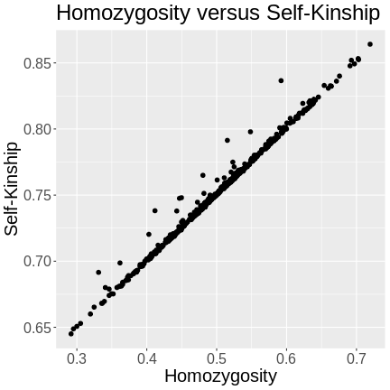
The kinship of a mouse with itself will only be 1 if the mouse is homozygous at every marker. Since the mice in this study are F2s, they will have genomes that are around 50% heterozygous. The variation in heterozygosity affects the actual kinship values, but, on average, we expect self-kinship to be 0.75 because half of the genome is homozygous and contributes values of 1, and half of the genome is heterozygous and contributes values of 0.5. So \((0.5 \times 1) + (0.5 \times 0.5) = 0.75\).
This is shown in the plot below of homozygosity versus kinship. There is a clear linear relationship between the two values and at 0.5 homozygosity, the self-kinship values is 0.75. The slope of the line is 0.5.
R
# 1 & 3 are the encodings for the two homozygous genotypes
homo <- sapply(cross$geno,
               function(z) {
                 rowSums(z == 1 | z == 3)
               })

homo <- rowSums(homo) / sum(n_mar(cross))

df   <- data.frame(id      = rownames(cross$geno[[1]]),
                   homo    = homo,
                   kinship = diag(kinship))

df |>
  ggplot(aes(homo, kinship)) +
    geom_point(size = 2) +
    labs(title = "Homozygosity versus Self-Kinship",
         x     = "Homozygosity",
         y     = "Self-Kinship") +
    theme(text = element_text(size = 20))

R
rm(homo, df)
- Kinship matrices account for relationships among individuals.
- Kinship is calculated as the proportion of shared alleles between individuals.
- Kinship calculation is a precursor to a genome scan via a linear mixed model.
